https://www.news-medical.net/health/Growing-an-eye-for-transplantation-potentials-and-pitfalls.aspx
https://www.sciencedirect.com/science/article/pii/S1818087621000337?utm_source=TrendMD&utm_medium=cpc&utm_campaign=_Asian_Journal_of_Pharmaceutical_Sciences_TrendMD_1
https://www.livescience.com/brain-organoid-optic-eyes.html
https://pubmed.ncbi.nlm.nih.gov/2271446/
https://abcnews.go.com/Technology/story?id=120075&page=1
https://www.nytimes.com/2020/06/29/science/flatworms-eyes-regeneration.html
https://neurosciencenews.com/retina-cells-in-dish-genetics-2081/
An image sensor or imager is a sensor that detects and conveys information used to form an image. It does so by converting the variable attenuation of light waves (as they pass through or reflect off objects) into signals, small bursts of current that convey the information. The waves can be light or other electromagnetic radiation. Image sensors are used in electronic imaging devices of both analog and digital types, which include digital cameras, camera modules, camera phones, optical mouse devices,[1][2][3] medical imaging equipment, night vision equipment such as thermal imaging devices, radar, sonar, and others. As technology changes, electronic and digital imaging tends to replace chemical and analog imaging.
The two main types of electronic image sensors are the charge-coupled device (CCD) and the active-pixel sensor (CMOS sensor). Both CCD and CMOS sensors are based on metal–oxide–semiconductor (MOS) technology, with CCDs based on MOS capacitors and CMOS sensors based on MOSFET (MOS field-effect transistor) amplifiers. Analog sensors for invisible radiation tend to involve vacuum tubes of various kinds, while digital sensors include flat-panel detectors. 
A micrograph of the corner of the photosensor array of a webcam digital camera
https://en.wikipedia.org/wiki/Image_sensor
Photodetectors, also called photosensors, are sensors of light or other electromagnetic radiation.[1] There is a wide variety of photodetectors which may be classified by mechanism of detection, such as photoelectric or photochemical effects, or by various performance metrics, such as spectral response. Semiconductor-based photodetectors typically photo detector have a p–n junction that converts light photons into current. The absorbed photons make electron–hole pairs in the depletion region. Photodiodes and photo transistors are a few examples of photo detectors. Solar cells convert some of the light energy absorbed into electrical energy.

A photodetector salvaged from a CD-ROM drive. The photodetector contains three photodiodes, visible in the photo (in center).
https://en.wikipedia.org/wiki/Photodetector
A photon (from Ancient Greek φῶς, φωτός (phôs, phōtós) 'light') is an elementary particle that is a quantum of the electromagnetic field, including electromagnetic radiation such as light and radio waves, and the force carrier for the electromagnetic force. Photons are massless,[a] so they always move at the speed of light in vacuum, 299792458 m/s (or about 186,282 mi/s). The photon belongs to the class of boson particles.
As with other elementary particles, photons are best explained by quantum mechanics and exhibit wave–particle duality, their behavior featuring properties of both waves and particles.[2] The modern photon concept originated during the first two decades of the 20th century with the work of Albert Einstein, who built upon the research of Max Planck. While trying to explain how matter and electromagnetic radiation could be in thermal equilibrium with one another, Planck proposed that the energy stored within a material object should be regarded as composed of an integer number of discrete, equal-sized parts. To explain the photoelectric effect, Einstein introduced the idea that light itself is made of discrete units of energy. In 1926, Gilbert N. Lewis popularized the term photon for these energy units.[3][4][5] Subsequently, many other experiments validated Einstein's approach.[6][7][8]
In the Standard Model of particle physics, photons and other elementary particles are described as a necessary consequence of physical laws having a certain symmetry at every point in spacetime. The intrinsic properties of particles, such as charge, mass, and spin, are determined by gauge symmetry. The photon concept has led to momentous advances in experimental and theoretical physics, including lasers, Bose–Einstein condensation, quantum field theory, and the probabilistic interpretation of quantum mechanics. It has been applied to photochemistry, high-resolution microscopy, and measurements of molecular distances. Moreover, photons have been studied as elements of quantum computers, and for applications in optical imaging and optical communication such as quantum cryptography.
Nomenclature
Photoelectric effect: the emission of electrons from a metal plate caused by light quanta – photons. 
1926 Gilbert N. Lewis letter which brought the word "photon" into common usage
The word quanta (singular quantum, Latin for how much) was used before 1900 to mean particles or amounts of different quantities, including electricity. In 1900, the German physicist Max Planck was studying black-body radiation, and he suggested that the experimental observations, specifically at shorter wavelengths, would be explained if the energy stored within a molecule was a "discrete quantity composed of an integral number of finite equal parts", which he called "energy elements".[9] In 1905, Albert Einstein published a paper in which he proposed that many light-related phenomena—including black-body radiation and the photoelectric effect—would be better explained by modelling electromagnetic waves as consisting of spatially localized, discrete wave-packets.[10] He called such a wave-packet a light quantum (German: ein Lichtquant).[b]
The name photon derives from the Greek word for light, φῶς (transliterated phôs). Arthur Compton used photon in 1928, referring to G.N. Lewis, who coined the term in a letter to Nature on 18 December 1926.[3][11] The same name was used earlier but was never widely adopted before Lewis: in 1916 by the American physicist and psychologist Leonard T. Troland, in 1921 by the Irish physicist Joly, in 1924 by the French physiologist René Wurmser (1890–1993), and in 1926 by the French physicist Frithiof Wolfers (1891–1971).[5] The name was suggested initially as a unit related to the illumination of the eye and the resulting sensation of light and was used later in a physiological context. Although Wolfers's and Lewis's theories were contradicted by many experiments and never accepted, the new name was adopted by most physicists very soon after Compton used it.[5][c]
In physics, a photon is usually denoted by the symbol γ (the Greek letter gamma). This symbol for the photon probably derives from gamma rays, which were discovered in 1900 by Paul Villard,[13][14] named by Ernest Rutherford in 1903, and shown to be a form of electromagnetic radiation in 1914 by Rutherford and Edward Andrade.[15] In chemistry and optical engineering, photons are usually symbolized by hν, which is the photon energy, where h is the Planck constant and the Greek letter ν (nu) is the photon's frequency.[16]
https://en.wikipedia.org/wiki/Photon
A p–n junction is a boundary or interface between two types of semiconductor materials, p-type and n-type, inside a single crystal of semiconductor. The "p" (positive) side contains an excess of holes, while the "n" (negative) side contains an excess of electrons in the outer shells of the electrically neutral atoms there. This allows electrical current to pass through the junction only in one direction. The p-n junction is created by doping, for example by ion implantation, diffusion of dopants, or by epitaxy (growing a layer of crystal doped with one type of dopant on top of a layer of crystal doped with another type of dopant). If two separate pieces of material were used, this would introduce a grain boundary between the semiconductors that would severely inhibit its utility by scattering the electrons and holes.[citation needed]
p–n junctions are elementary "building blocks" of semiconductor electronic devices such as diodes, transistors, solar cells, light-emitting diodes (LEDs), and integrated circuits; they are the active sites where the electronic action of the device takes place. For example, a common type of transistor, the bipolar junction transistor (BJT), consists of two p–n junctions in series, in the form n–p–n or p–n–p; while a diode can be made from a single p-n junction. A Schottky junction is a special case of a p–n junction, where metal serves the role of the n-type semiconductor.

A p–n junction. The circuit symbol is shown: the triangle corresponds to the p side.
https://en.wikipedia.org/wiki/P%E2%80%93n_junction
Ion implantation is a low-temperature process by which ions of one element are accelerated into a solid target, thereby changing the physical, chemical, or electrical properties of the target. Ion implantation is used in semiconductor device fabrication and in metal finishing, as well as in materials science research. The ions can alter the elemental composition of the target (if the ions differ in composition from the target) if they stop and remain in the target. Ion implantation also causes chemical and physical changes when the ions impinge on the target at high energy. The crystal structure of the target can be damaged or even destroyed by the energetic collision cascades, and ions of sufficiently high energy (tens of MeV) can cause nuclear transmutation.
General principle
Ion implantation setup with mass separator
Ion implantation equipment typically consists of an ion source, where ions of the desired element are produced, an accelerator, where the ions are electrostatically accelerated to a high energy or using radiofrequency, and a target chamber, where the ions impinge on a target, which is the material to be implanted. Thus ion implantation is a special case of particle radiation. Each ion is typically a single atom or molecule, and thus the actual amount of material implanted in the target is the integral over time of the ion current. This amount is called the dose. The currents supplied by implants are typically small (micro-amperes), and thus the dose which can be implanted in a reasonable amount of time is small. Therefore, ion implantation finds application in cases where the amount of chemical change required is small.
Typical ion energies are in the range of 10 to 500 keV (1,600 to 80,000 aJ). Energies in the range 1 to 10 keV (160 to 1,600 aJ) can be used, but result in a penetration of only a few nanometers or less. Energies lower than this result in very little damage to the target, and fall under the designation ion beam deposition. Higher energies can also be used: accelerators capable of 5 MeV (800,000 aJ) are common. However, there is often great structural damage to the target, and because the depth distribution is broad (Bragg peak), the net composition change at any point in the target will be small.
The energy of the ions, as well as the ion species and the composition of the target determine the depth of penetration of the ions in the solid: A monoenergetic ion beam will generally have a broad depth distribution. The average penetration depth is called the range of the ions. Under typical circumstances ion ranges will be between 10 nanometers and 1 micrometer. Thus, ion implantation is especially useful in cases where the chemical or structural change is desired to be near the surface of the target. Ions gradually lose their energy as they travel through the solid, both from occasional collisions with target atoms (which cause abrupt energy transfers) and from a mild drag from overlap of electron orbitals, which is a continuous process. The loss of ion energy in the target is called stopping and can be simulated with the binary collision approximation method.
Accelerator systems for ion implantation are generally classified into medium current (ion beam currents between 10 μA and ~2 mA), high current (ion beam currents up to ~30 mA), high energy (ion energies above 200 keV and up to 10 MeV), and very high dose (efficient implant of dose greater than 1016 ions/cm2).[1]
https://en.wikipedia.org/wiki/Ion_implantation
Properties
This section needs additional citations for verification. Please help improve this article by adding citations to reliable sources in this section. Unsourced material may be challenged and removed. (May 2022) (Learn how and when to remove this template message)![]()
This section may be too technical for most readers to understand. Please help improve it to make it understandable to non-experts, without removing the technical details. (May 2022) (Learn how and when to remove this template message)
Silicon atoms (Si) enlarged about 45,000,000x.
The p–n junction possesses a useful property for modern semiconductor electronics. A p-doped semiconductor is relatively conductive. The same is true of an n-doped semiconductor, but the junction between them can become depleted of charge carriers, and hence non-conductive, depending on the relative voltages of the two semiconductor regions. By manipulating this non-conductive layer, p–n junctions are commonly used as diodes: circuit elements that allow a flow of electricity in one direction but not in the other (opposite) direction.
Bias is the application of a voltage relative to a p–n junction region: forward bias is in the direction of easy current flow
reverse bias is in the direction of little or no current flow.
The forward-bias and the reverse-bias properties of the p–n junction imply that it can be used as a diode. A p–n junction diode allows electric charges to flow in one direction, but not in the opposite direction; negative charges (electrons) can easily flow through the junction from n to p but not from p to n, and the reverse is true for holes. When the p–n junction is forward-biased, electric charge flows freely due to reduced resistance of the p–n junction. When the p–n junction is reverse-biased, however, the junction barrier (and therefore resistance) becomes greater and charge flow is minimal.
https://en.wikipedia.org/wiki/P%E2%80%93n_junction
Types
A commercial amplified photodetector for use in optics research
Photodetectors may be classified by their mechanism for detection:[2][unreliable source?][3][4] Photoemission or photoelectric effect: Photons cause electrons to transition from the conduction band of a material to free electrons in a vacuum or gas.
Thermal: Photons cause electrons to transition to mid-gap states then decay back to lower bands, inducing phonon generation and thus heat.
Polarization: Photons induce changes in polarization states of suitable materials, which may lead to change in index of refraction or other polarization effects.
Photochemical: Photons induce a chemical change in a material.
Weak interaction effects: photons induce secondary effects such as in photon drag[5][6] detectors or gas pressure changes in Golay cells.
Photodetectors may be used in different configurations. Single sensors may detect overall light levels. A 1-D array of photodetectors, as in a spectrophotometer or a Line scanner, may be used to measure the distribution of light along a line. A 2-D array of photodetectors may be used as an image sensor to form images from the pattern of light before it.
A photodetector or array is typically covered by an illumination window, sometimes having an anti-reflective coating.
Properties
There are a number of performance metrics, also called figures of merit, by which photodetectors are characterized and compared[2][3] Spectral response: The response of a photodetector as a function of photon frequency.
Quantum efficiency: The number of carriers (electrons or holes) generated per photon.
Responsivity: The output current divided by total light power falling upon the photodetector.
Noise-equivalent power: The amount of light power needed to generate a signal comparable in size to the noise of the device.
Detectivity: The square root of the detector area divided by the noise equivalent power.
Gain: The output current of a photodetector divided by the current directly produced by the photons incident on the detectors, i.e., the built-in current gain.
Dark current: The current flowing through a photodetector even in the absence of light.
Response time: The time needed for a photodetector to go from 10% to 90% of final output.
Noise spectrum: The intrinsic noise voltage or current as a function of frequency. This can be represented in the form of a noise spectral density.
Nonlinearity: The RF-output is limited by the nonlinearity of the photodetector[7]
Devices
Grouped by mechanism, photodetectors include the following devices:
Photoemission or photoelectricGaseous ionization detectors are used in experimental particle physics to detect photons and particles with sufficient energy to ionize gas atoms or molecules. Electrons and ions generated by ionization cause a current flow which can be measured.
Photomultiplier tubes containing a photocathode which emits electrons when illuminated, the electrons are then amplified by a chain of dynodes.
Phototubes containing a photocathode which emits electrons when illuminated, such that the tube conducts a current proportional to the light intensity.
Microchannel plate detectors use a porous glass substrate as a mechanism for multiplying electrons. They can be used in combination with a photocathode like the photomultiplier described above, with the porous glass substrate acting as a dynode stage
SemiconductorActive-pixel sensors (APSs) are image sensors. Usually made in a complementary metal–oxide–semiconductor (CMOS) process, and also known as CMOS image sensors, APSs are commonly used in cell phone cameras, web cameras, and some DSLRs.
Cadmium zinc telluride radiation detectors can operate in direct-conversion (or photoconductive) mode at room temperature, unlike some other materials (particularly germanium) which require liquid nitrogen cooling. Their relative advantages include high sensitivity for x-rays and gamma-rays, due to the high atomic numbers of Cd and Te, and better energy resolution than scintillator detectors.
Charge-coupled devices (CCD) are image sensors which are used to record images in astronomy, digital photography, and digital cinematography. Before the 1990s, photographic plates were most common in astronomy. The next generation of astronomical instruments, such as the Astro-E2, include cryogenic detectors.
HgCdTe infrared detectors. Detection occurs when an infrared photon of sufficient energy kicks an electron from the valence band to the conduction band. Such an electron is collected by a suitable external readout integrated circuits (ROIC) and transformed into an electric signal.
LEDs which are reverse-biased to act as photodiodes. See LEDs as photodiode light sensors.
Photoresistors or Light Dependent Resistors (LDR) which change resistance according to light intensity. Normally the resistance of LDRs decreases with increasing intensity of light falling on it.[8]
Photodiodes which can operate in photovoltaic mode or photoconductive mode.[9][10] Photodiodes are often combined with low-noise analog electronics to convert the photocurrent into a voltage that can be digitized.[11][12]
Phototransistors, which act like amplifying photodiodes.
Pinned photodiodes, a photodetector structure with low lag, low noise, high quantum efficiency, and low dark current, widely used in most CCD and CMOS image sensors.[13]
Quantum dot photoconductors or photodiodes, which can handle wavelengths in the visible and infrared spectral regions.
Semiconductor detectors are employed in gamma and X-ray spectrometry and as particle detectors.[citation needed]
Silicon drift detectors (SDDs) are X-ray radiation detectors used in x-ray spectrometry (EDS) and electron microscopy (EDX).[14]
PhotovoltaicPhotovoltaic cells or solar cells which produce a voltage and supply an electric current when sunlight or certain kinds of light shines on them.
ThermalBolometers measure the power of incident electromagnetic radiation via the heating of a material with a temperature-dependent electrical resistance. A microbolometer is a specific type of bolometer used as a detector in a thermal camera.
Cryogenic detectors are sufficiently sensitive to measure the energy of single x-ray, visible and infrared photons.[15]
Pyroelectric detectors detect photons through the heat they generate and the subsequent voltage generated in pyroelectric materials.
Thermopiles detect electromagnetic radiation through heat, then generating a voltage in thermocouples.
Golay cells detect photons by the heat they generate in a gas-filled chamber, causing the gas to expand and deform a flexible membrane whose deflection is measured.
PhotochemicalPhotoreceptor cells in the retina detect light through, for instance, a rhodopsin photon-induced chemical cascade.
Chemical detectors, such as photographic plates, in which a silver halide molecule is split into an atom of metallic silver and a halogen atom. The photographic developer causes adjacent molecules to split similarly.
PolarizationThe photorefractive effect is used in holographic data storage.
Polarization-sensitive photodetectors use optically anisotropic materials to detect photons of a desired linear polarization.[16]
Graphene/silicon photodetectors
A graphene/n-type silicon heterojunction has been demonstrated to exhibit strong rectifying behavior and high photoresponsivity. Graphene is coupled with silicon quantum dots (Si QDs) on top of bulk Si to form a hybrid photodetector. Si QDs cause an increase of the built-in potential of the graphene/Si Schottky junction while reducing the optical reflection of the photodetector. Both the electrical and optical contributions of Si QDs enable a superior performance of the photodetector.[17]
Frequency range
In 2014 a technique for extending semiconductor-based photodetector's frequency range to longer, lower-energy wavelengths. Adding a light source to the device effectively "primed" the detector so that in the presence of long wavelengths, it fired on wavelengths that otherwise lacked the energy to do so.[18]
See alsoLighting control system
List of sensors
Optoelectronics
Photoelectric sensor
Photosensitivity
Readout integrated circuit
Resonant-cavity-enhanced photo detector
Photodetection
Authority control: National ![]()
Germany
Czech Republic 2
Category: Photodetectors
Electronic components
Semiconductor
devices
MOS
transistors
Transistor
NMOS
PMOS
BiCMOS
BioFET
Chemical field-effect transistor (ChemFET)
Complementary MOS (CMOS)
Depletion-load NMOS
Fin field-effect transistor (FinFET)
Floating-gate MOSFET (FGMOS)
Insulated-gate bipolar transistor (IGBT)
ISFET
LDMOS
MOS field-effect transistor (MOSFET)
Multi-gate field-effect transistor (MuGFET)
Power MOSFET
Thin-film transistor (TFT)
VMOS
UMOS
Other
transistors
Bipolar junction transistor (BJT)
Darlington transistor
Diffused junction transistor
Field-effect transistor (FET) Junction Gate FET (JFET)
Organic FET (OFET)
Light-emitting transistor (LET) Organic LET (OLET)
Pentode transistor
Point-contact transistor
Programmable unijunction transistor (PUT)
Static induction transistor (SIT)
Tetrode transistor
Unijunction transistor (UJT)
Diodes
Avalanche diode
Constant-current diode (CLD, CRD)
Gunn diode
Laser diode (LD)
Light-emitting diode (LED)
Organic light-emitting diode (OLED)
Photodiode
PIN diode
Schottky diode
Step recovery diode
Zener diode
Other
devices
Printed electronics
Printed circuit board
DIAC
Heterostructure barrier varactor
Integrated circuit (IC)
Hybrid integrated circuit
Light emitting capacitor (LEC)
Memistor
Memristor
Memtransistor
Memory cell
Metal oxide varistor (MOV)
Mixed-signal integrated circuit
MOS integrated circuit (MOS IC)
Organic semiconductor
Photodetector
Quantum circuit
RF CMOS
Silicon controlled rectifier (SCR)
Solaristor
Static induction thyristor (SITh)
Three-dimensional integrated circuit (3D IC)
Thyristor
Trancitor
TRIAC
Varicap
Voltage regulators
Linear regulator
Low-dropout regulator
Switching regulator
Buck
Boost
Buck–boost
Split-pi
Ćuk
SEPIC
Charge pump
Switched capacitor
Vacuum tubes
Acorn tube
Audion
Beam tetrode
Barretter
Compactron
Diode
Fleming valve
Neutron tube
Nonode
Nuvistor
Pentagrid (Hexode, Heptode, Octode)
Pentode
Photomultiplier
Phototube
Tetrode
Triode
Vacuum tubes (RF)
Backward-wave oscillator (BWO)
Cavity magnetron
Crossed-field amplifier (CFA)
Gyrotron
Inductive output tube (IOT)
Klystron
Maser
Sutton tube
Traveling-wave tube (TWT)
X-ray tube
Cathode-ray tubes
Beam deflection tube
Charactron
Iconoscope
Magic eye tube
Monoscope
Selectron tube
Storage tube
Trochotron
Video camera tube
Williams tube
Gas-filled tubes
Cold cathode
Crossatron
Dekatron
Ignitron
Krytron
Mercury-arc valve
Neon lamp
Nixie tube
Thyratron
Trigatron
Voltage-regulator tube
Adjustable
Potentiometer digital
Variable capacitor
Varicap
Passive
Connector audio and video
electrical power
RF
Electrolytic detector
Ferrite
Antifuse
Fuse resettable
eFUSE
Resistor
Switch
Thermistor
Transformer
Varistor
Wire Wollaston wire
Reactive
Capacitor types
Ceramic resonator
Crystal oscillator
Inductor
Parametron
Relay reed relay
mercury relay
https://en.wikipedia.org/wiki/Photodetector
CCD vs. CMOS sensors
A micrograph of the corner of the photosensor array of a webcam digital camera 
Image sensor (upper left) on the motherboard of a Nikon Coolpix L2 6 MP
The two main types of digital image sensors are the charge-coupled device (CCD) and the active-pixel sensor (CMOS sensor), fabricated in complementary MOS (CMOS) or N-type MOS (NMOS or Live MOS) technologies. Both CCD and CMOS sensors are based on the MOS technology,[4] with MOS capacitors being the building blocks of a CCD,[5] and MOSFET amplifiers being the building blocks of a CMOS sensor.[6][7]
Cameras integrated in small consumer products generally use CMOS sensors, which are usually cheaper and have lower power consumption in battery powered devices than CCDs.[8] CCD sensors are used for high end broadcast quality video cameras, and CMOS sensors dominate in still photography and consumer goods where overall cost is a major concern. Both types of sensor accomplish the same task of capturing light and converting it into electrical signals.[citation needed]
Each cell of a CCD image sensor is an analog device. When light strikes the chip it is held as a small electrical charge in each photo sensor. The charges in the line of pixels nearest to the (one or more) output amplifiers are amplified and output, then each line of pixels shifts its charges one line closer to the amplifiers, filling the empty line closest to the amplifiers. This process is then repeated until all the lines of pixels have had their charge amplified and output.[9]
A CMOS image sensor has an amplifier for each pixel compared to the few amplifiers of a CCD. This results in less area for the capture of photons than a CCD, but this problem has been overcome by using microlenses in front of each photodiode, which focus light into the photodiode that would have otherwise hit the amplifier and not been detected.[9] Some CMOS imaging sensors also use Back-side illumination to increase the number of photons that hit the photodiode.[10] CMOS sensors can potentially be implemented with fewer components, use less power, and/or provide faster readout than CCD sensors.[11] They are also less vulnerable to static electricity discharges.
Another design, a hybrid CCD/CMOS architecture (sold under the name "sCMOS") consists of CMOS readout integrated circuits (ROICs) that are bump bonded to a CCD imaging substrate – a technology that was developed for infrared staring arrays and has been adapted to silicon-based detector technology.[12] Another approach is to utilize the very fine dimensions available in modern CMOS technology to implement a CCD like structure entirely in CMOS technology: such structures can be achieved by separating individual poly-silicon gates by a very small gap; though still a product of research hybrid sensors can potentially harness the benefits of both CCD and CMOS imagers.[13]
Performance
See also: EMVA1288
There are many parameters that can be used to evaluate the performance of an image sensor, including dynamic range, signal-to-noise ratio, and low-light sensitivity. For sensors of comparable types, the signal-to-noise ratio and dynamic range improve as the size increases. It’s because in a given integration (exposure) time, more photons hit the pixel with larger area.
Exposure-time control
Exposure time of image sensors is generally controlled by either a conventional mechanical shutter, as in film cameras, or by an electronic shutter. Electronic shuttering can be "global," in which case the entire image sensor area's accumulation of photoelectrons starts and stops simultaneously, or "rolling" in which case the exposure interval of each row immediate precedes that row's readout, in a process that "rolls" across the image frame (typically from top to bottom in landscape format). Global electronic shuttering is less common, as it requires "storage" circuits to hold charge from the end of the exposure interval until the readout process gets there, typically a few milliseconds later.[14]
Color separation
Bayer pattern on sensor 
Foveon's scheme of vertical filtering for color sensing
There are several main types of color image sensors, differing by the type of color-separation mechanism: Integral color sensors[15] use a color filter array fabricated on top of a single monochrome CCD or CMOS image sensor. The most common color filter array pattern, the Bayer pattern, uses a checkerboard arrangement of two green pixels for each red and blue pixel, although many other color filter patterns have been developed, including patterns using cyan, magenta, yellow, and white pixels.[16] Integral color sensors were initially manufactured by transferring colored dyes through photoresist windows onto a polymer receiving layer coated on top of a monochrome CCD sensor.[17] Since each pixel provides only a single color (such as green), the "missing" color values (such as red and blue) for the pixel are interpolated using neighboring pixels.[18] This processing is also referred to as demosaicing or de-bayering.
Foveon X3 sensor, using an array of layered pixel sensors, separating light via the inherent wavelength-dependent absorption property of silicon, such that every location senses all three color channels. This method is similar to how color film for photography works.
3CCD, using three discrete image sensors, with the color separation done by a dichroic prism. The dichroic elements provide a sharper color separation, thus improving color quality. Because each sensor is equally sensitive within its passband, and at full resolution, 3-CCD sensors produce better color quality and better low light performance. 3-CCD sensors produce a full 4:4:4 signal, which is preferred in television broadcasting, video editing and chroma key visual effects.
Specialty sensors
Infrared view of the Orion Nebula taken by ESO's HAWK-I, a cryogenic wide-field imager[19]
Special sensors are used in various applications such as thermography, creation of multi-spectral images, video laryngoscopes, gamma cameras, sensor arrays for x-rays, and other highly sensitive arrays for astronomy.[20]
While in general, digital cameras use a flat sensor, Sony prototyped a curved sensor in 2014 to reduce/eliminate Petzval field curvature that occurs with a flat sensor. Use of a curved sensor allows a shorter and smaller diameter of the lens with reduced elements and components with greater aperture and reduced light fall-off at the edge of the photo.[21]
https://en.wikipedia.org/wiki/Image_sensor
History
See also: Digital imaging
Early analog sensors for visible light were video camera tubes. They date back to the 1930s, and several types were developed up until the 1980s. By the early 1990s, they had been replaced by modern solid-state CCD image sensors.[22]
The basis for modern solid-state image sensors is MOS technology,[23][24] which originates from the invention of the MOSFET by Mohamed M. Atalla and Dawon Kahng at Bell Labs in 1959.[25] Later research on MOS technology led to the development of solid-state semiconductor image sensors, including the charge-coupled device (CCD) and later the active-pixel sensor (CMOS sensor).[23][24]
The passive-pixel sensor (PPS) was the precursor to the active-pixel sensor (APS).[7] A PPS consists of passive pixels which are read out without amplification, with each pixel consisting of a photodiode and a MOSFET switch.[26] It is a type of photodiode array, with pixels containing a p-n junction, integrated capacitor, and MOSFETs as selection transistors. A photodiode array was proposed by G. Weckler in 1968.[6] This was the basis for the PPS.[7] These early photodiode arrays were complex and impractical, requiring selection transistors to be fabricated within each pixel, along with on-chip multiplexer circuits. The noise of photodiode arrays was also a limitation to performance, as the photodiode readout bus capacitance resulted in increased noise level. Correlated double sampling (CDS) could also not be used with a photodiode array without external memory.[6] However, in 1914 Deputy Consul General Carl R. Loop, reported to the state department in a Consular Report on Archibald M. Low's Televista system that "It is stated that the selenium in the transmitting screen may be replaced by any diamagnetic material".[27]
In June 2022, Samsung Electronics announced that it had created a 200 million pixel image sensor. The 200MP ISOCELL HP3 has 0.56 micrometer pixels with Samsung reporting that previous sensors had 0.64 micrometer pixels, a 12% decrease since 2019. The new sensor contains 200 million pixels in a 2 x 1.4 inch lens.[28]
Charge-coupled device
Main article: Charge-coupled device
The charge-coupled device (CCD) was invented by Willard S. Boyle and George E. Smith at Bell Labs in 1969.[29] While researching MOS technology, they realized that an electric charge was the analogy of the magnetic bubble and that it could be stored on a tiny MOS capacitor. As it was fairly straightforward to fabricate a series of MOS capacitors in a row, they connected a suitable voltage to them so that the charge could be stepped along from one to the next.[23] The CCD is a semiconductor circuit that was later used in the first digital video cameras for television broadcasting.[30]
Early CCD sensors suffered from shutter lag. This was largely resolved with the invention of the pinned photodiode (PPD).[7] It was invented by Nobukazu Teranishi, Hiromitsu Shiraki and Yasuo Ishihara at NEC in 1980.[7][31] It was a photodetector structure with low lag, low noise, high quantum efficiency and low dark current.[7] In 1987, the PPD began to be incorporated into most CCD devices, becoming a fixture in consumer electronic video cameras and then digital still cameras. Since then, the PPD has been used in nearly all CCD sensors and then CMOS sensors.[7]
Active-pixel sensor
Main article: Active-pixel sensor
The NMOS active-pixel sensor (APS) was invented by Olympus in Japan during the mid-1980s. This was enabled by advances in MOS semiconductor device fabrication, with MOSFET scaling reaching smaller micron and then sub-micron levels.[6][32] The first NMOS APS was fabricated by Tsutomu Nakamura's team at Olympus in 1985.[33] The CMOS active-pixel sensor (CMOS sensor) was later improved by a group of scientists at the NASA Jet Propulsion Laboratory in 1993.[7] By 2007, sales of CMOS sensors had surpassed CCD sensors.[34] By the 2010s, CMOS sensors largely displaced CCD sensors in all new applications.
Other image sensors
The first commercial digital camera, the Cromemco Cyclops in 1975, used a 32×32 MOS image sensor. It was a modified MOS dynamic RAM (DRAM) memory chip.[35]
MOS image sensors are widely used in optical mouse technology. The first optical mouse, invented by Richard F. Lyon at Xerox in 1980, used a 5 µm NMOS integrated circuit sensor chip.[36][37] Since the first commercial optical mouse, the IntelliMouse introduced in 1999, most optical mouse devices use CMOS sensors.[38]
In February 2018, researchers at Dartmouth College announced a new image sensing technology that the researchers call QIS, for Quanta Image Sensor. Instead of pixels, QIS chips have what the researchers call "jots." Each jot can detect a single particle of light, called a photon.[39]
See alsoList of sensors used in digital cameras
Contact image sensor (CIS)
Electro-optical sensor
Video camera tube
Semiconductor detector
Fill factor
Full-frame digital SLR
Image resolution
Image sensor format, the sizes and shapes of common image sensors
Color filter array, mosaic of tiny color filters over color image sensors
Sensitometry, the scientific study of light-sensitive materials
History of television, the development of electronic imaging technology since the 1880s
List of large sensor interchangeable-lens video cameras
Oversampled binary image sensor
Computer vision
Push broom scanner
Whisk broom scanner
https://en.wikipedia.org/wiki/Image_sensor
Digital imaging or digital image acquisition is the creation of a digital representation of the visual characteristics of an object,[1] such as a physical scene or the interior structure of an object. The term is often assumed to imply or include the processing, compression, storage, printing and display of such images. A key advantage of a digital image, versus an analog image such as a film photograph, is the ability to digitally propagate copies of the original subject indefinitely without any loss of image quality.
Digital imaging can be classified by the type of electromagnetic radiation or other waves whose variable attenuation, as they pass through or reflect off objects, conveys the information that constitutes the image. In all classes of digital imaging, the information is converted by image sensors into digital signals that are processed by a computer and made output as a visible-light image. For example, the medium of visible light allows digital photography (including digital videography) with various kinds of digital cameras (including digital video cameras). X-rays allow digital X-ray imaging (digital radiography, fluoroscopy, and CT), and gamma rays allow digital gamma ray imaging (digital scintigraphy, SPECT, and PET). Sound allows ultrasonography (such as medical ultrasonography) and sonar, and radio waves allow radar. Digital imaging lends itself well to image analysis by software, as well as to image editing (including image manipulation).
History
Before digital imaging, the first photograph ever produced, View from the Window at Le Gras, was in 1826 by Frenchman Joseph Nicéphore Niépce. When Joseph was 28, he was discussing with his brother Claude about the possibility of reproducing images with light. His focus on his new innovations began in 1816. He was in fact more interested in creating an engine for a boat. Joseph and his brother focused on that for quite some time and Claude successfully promoted his innovation moving and advancing him to England. Joseph was able to focus on the photograph and finally in 1826, he was able to produce his first photograph of a view through his window. This took 8 hours or more of exposure to light.[2]
The first digital image was produced in 1920, by the Bartlane cable picture transmission system. British inventors, Harry G. Bartholomew and Maynard D. McFarlane, developed this method. The process consisted of “a series of negatives on zinc plates that were exposed for varying lengths of time, thus producing varying densities,”.[3] The Bartlane cable picture transmission system generated at both its transmitter and its receiver end a punched data card or tape that was recreated as an image.[4]
In 1957, Russell A. Kirsch produced a device that generated digital data that could be stored in a computer; this used a drum scanner and photomultiplier tube.[3]
Digital imaging was developed in the 1960s and 1970s, largely to avoid the operational weaknesses of film cameras, for scientific and military missions including the KH-11 program. As digital technology became cheaper in later decades, it replaced the old film methods for many purposes.
In the early 1960s, while developing compact, lightweight, portable equipment for the onboard nondestructive testing of naval aircraft, Frederick G. Weighart[5] and James F. McNulty (U.S. radio engineer)[6] at Automation Industries, Inc., then, in El Segundo, California co-invented the first apparatus to generate a digital image in real-time, which image was a fluoroscopic digital radiograph. Square wave signals were detected on the fluorescent screen of a fluoroscope to create the image.
Digital image sensors
Main article: Image sensor
The charge-coupled device was invented by Willard S. Boyle and George E. Smith at Bell Labs in 1969.[7] While researching MOS technology, they realized that an electric charge was the analogy of the magnetic bubble and that it could be stored on a tiny MOS capacitor. As it was fairly straightforward to fabricate a series of MOS capacitors in a row, they connected a suitable voltage to them so that the charge could be stepped along from one to the next.[8] The CCD is a semiconductor circuit that was later used in the first digital video cameras for television broadcasting.[9]
Early CCD sensors suffered from shutter lag. This was largely resolved with the invention of the pinned photodiode (PPD).[10] It was invented by Nobukazu Teranishi, Hiromitsu Shiraki and Yasuo Ishihara at NEC in 1980.[10][11] It was a photodetector structure with low lag, low noise, high quantum efficiency and low dark current.[10] In 1987, the PPD began to be incorporated into most CCD devices, becoming a fixture in consumer electronic video cameras and then digital still cameras. Since then, the PPD has been used in nearly all CCD sensors and then CMOS sensors.[10]
The NMOS active-pixel sensor (APS) was invented by Olympus in Japan during the mid-1980s. This was enabled by advances in MOS semiconductor device fabrication, with MOSFET scaling reaching smaller micron and then sub-micron levels.[12][13] The NMOS APS was fabricated by Tsutomu Nakamura's team at Olympus in 1985.[14] The CMOS active-pixel sensor (CMOS sensor) was later developed by Eric Fossum's team at the NASA Jet Propulsion Laboratory in 1993.[10] By 2007, sales of CMOS sensors had surpassed CCD sensors.[15]
Digital image compression
Main article: Image compression
An important development in digital image compression technology was the discrete cosine transform (DCT).[16] DCT compression is used in JPEG, which was introduced by the Joint Photographic Experts Group in 1992.[17] JPEG compresses images down to much smaller file sizes, and has become the most widely used image file format on the Internet.[18]
Digital cameras
Main article: Digital camera
These different scanning ideas were the basis of the first designs of digital camera. Early cameras took a long time to capture an image and were poorly suited for consumer purposes.[3] It wasn't until the adoption of the CCD (charge-coupled device) that the digital camera really took off. The CCD became part of the imaging systems used in telescopes, the first black-and-white digital cameras in the 1980s.[3] Color was eventually added to the CCD and is a usual feature of cameras today.
Changing environment
Great strides have been made in the field of digital imaging. Negatives and exposure are foreign concepts to many, and the first digital image in 1920 led eventually to cheaper equipment, increasingly powerful yet simple software, and the growth of the Internet.[19]
The constant advancement and production of physical equipment and hardware related to digital imaging has affected the environment surrounding the field. From cameras and webcams to printers and scanners, the hardware is becoming sleeker, thinner, faster, and cheaper. As the cost of equipment decreases, the market for new enthusiasts widens, allowing more consumers to experience the thrill of creating their own images.
Everyday personal laptops, family desktops, and company computers are able to handle photographic software. Our computers are more powerful machines with increasing capacities for running programs of any kind—especially digital imaging software. And that software is quickly becoming both smarter and simpler. Although functions on today's programs reach the level of precise editing and even rendering 3-D images, user interfaces are designed to be friendly to advanced users as well as first-time fans.
The Internet allows editing, viewing, and sharing digital photos and graphics. A quick browse around the web can easily turn up graphic artwork from budding artists, news photos from around the world, corporate images of new products and services, and much more. The Internet has clearly proven itself a catalyst in fostering the growth of digital imaging.
Online photo sharing of images changes the way we understand photography and photographers. Online sites such as Flickr, Shutterfly, and Instagram give billions the capability to share their photography, whether they are amateurs or professionals. Photography has gone from being a luxury medium of communication and sharing to more of a fleeting moment in time. Subjects have also changed. Pictures used to be primarily taken of people and family. Now, we take them of anything. We can document our day and share it with everyone with the touch of our fingers.[20]
In 1826 Niepce was the first to develop a photo which used lights to reproduce images, the advancement of photography has drastically increased over the years. Everyone is now a photographer in their own way, whereas during the early 1800s and 1900s the expense of lasting photos was highly valued and appreciated by consumers and producers. According to the magazine article on five ways digital camera changed us states the following:The impact on professional photographers has been dramatic. Once upon a time a photographer wouldn't dare waste a shot unless they were virtually certain it would work.”The use of digital imaging( photography) has changed the way we interacted with our environment over the years. Part of the world is experienced differently through visual imagining of lasting memories, it has become a new form of communication with friends, family and love ones around the world without face to face interactions. Through photography it is easy to see those that you have never seen before and feel their presence without them being around, for example Instagram is a form of social media where anyone is allowed to shoot, edit, and share photos of whatever they want with friends and family. Facebook, snapshot, vine and twitter are also ways people express themselves with little or no words and are able to capture every moment that is important. Lasting memories that were hard to capture, is now easy because everyone is now able to take pictures and edit it on their phones or laptops. Photography has become a new way to communicate and it is rapidly increasing as time goes by, which has affected the world around us.[21]
A study done by Basey, Maines, Francis, and Melbourne found that drawings used in class have a significant negative effect on lower-order content for student's lab reports, perspectives of labs, excitement, and time efficiency of learning. Documentation style learning has no significant effects on students in these areas. He also found that students were more motivated and excited to learn when using digital imaging.[22]
Field advancements
In the field of education. As digital projectors, screens, and graphics find their way to the classroom, teachers and students alike are benefitting from the increased convenience and communication they provide, although their theft can be a common problem in schools.[23] In addition acquiring a basic digital imaging education is becoming increasingly important for young professionals. Reed, a design production expert from Western Washington University, stressed the importance of using “digital concepts to familiarize students with the exciting and rewarding technologies found in one of the major industries of the 21st century”.[24]
The field of medical imaging A branch of digital imaging that seeks to assist in the diagnosis and treatment of diseases, is growing at a rapid rate. A recent study by the American Academy of Pediatrics suggests that proper imaging of children who may have appendicitis may reduce the amount of appendectomies needed. Further advancements include amazingly detailed and accurate imaging of the brain, lungs, tendons, and other parts of the body—images that can be used by health professionals to better serve patients.[25]
According to Vidar, as more countries take on this new way of capturing an image, it has been found that image digitalization in medicine has been increasingly beneficial for both patient and medical staff. Positive ramifications of going paperless and heading towards digitization includes the overall reduction of cost in medical care, as well as an increased global, real-time, accessibility of these images. (http://www.vidar.com/film/images/stories/PDFs/newsroom/Digital%20Transition%20White%20Paper%20hi-res%20GFIN.pdf)
There is a program called Digital Imaging in Communications and Medicine (DICOM) that is changing the medical world as we know it. DICOM is not only a system for taking high quality images of the aforementioned internal organs, but also is helpful in processing those images. It is a universal system that incorporates image processing, sharing, and analyzing for the convenience of patient comfort and understanding. This service is all encompassing and is beginning a necessity.[26]
In the field of technology, digital image processing has become more useful than analog image processing when considering the modern technological advancement. Image sharpen & reinstatement – Image sharpens & reinstatement is the procedure of images which is capture by the contemporary camera making them an improved picture or manipulating the pictures in the way to get chosen product. This comprises the zooming process, the blurring process, the sharpening process, the gray scale to color translation process, the picture recovery process and the picture identification process.
Facial Recognition – Face recognition is a PC innovation that decides the positions and sizes of human faces in self-assertive digital pictures. It distinguishes facial components and overlooks whatever, for example, structures, trees & bodies.
Remote detection – Remote detecting is little or substantial scale procurement of data of article or occurrence, with the utilization of recording or ongoing detecting apparatus which is not in substantial or close contact with an article. Practically speaking, remote detecting is face-off accumulation using an assortment of gadgets for collecting data on particular article or location.
Pattern detection – The pattern detection is the study or investigation from picture processing. In the pattern detection, image processing is utilized for recognizing elements in the images and after that machine study is utilized to instruct a framework for variation in pattern. The pattern detection is utilized in computer-aided analysis, detection of calligraphy, identification of images, and many more.
Color processing – The color processing comprises processing of colored pictures and diverse color locations which are utilized. This moreover involves study of transmit, store, and encode of the color pictures.
Theoretical application
Although theories are quickly becoming realities in today's technological society, the range of possibilities for digital imaging is wide open. One major application that is still in the works is that of child safety and protection. How can we use digital imaging to better protect our kids? Kodak’s program, Kids Identification Digital Software (KIDS) may answer that question. The beginnings include a digital imaging kit to be used to compile student identification photos, which would be useful during medical emergencies and crimes. More powerful and advanced versions of applications such as these are still developing, with increased features constantly being tested and added.[27]
But parents and schools aren’t the only ones who see benefits in databases such as these. Criminal investigation offices, such as police precincts, state crime labs, and even federal bureaus have realized the importance of digital imaging in analyzing fingerprints and evidence, making arrests, and maintaining safe communities. As the field of digital imaging evolves, so does our ability to protect the public.[28]
Digital imaging can be closely related to the social presence theory especially when referring to the social media aspect of images captured by our phones. There are many different definitions of the social presence theory but two that clearly define what it is would be "the degree to which people are perceived as real" (Gunawardena, 1995), and "the ability to project themselves socially and emotionally as real people" (Garrison, 2000). Digital imaging allows one to manifest their social life through images in order to give the sense of their presence to the virtual world. The presence of those images acts as an extension of oneself to others, giving a digital representation of what it is they are doing and who they are with. Digital imaging in the sense of cameras on phones helps facilitate this effect of presence with friends on social media. Alexander (2012) states, "presence and representation is deeply engraved into our reflections on images...this is, of course, an altered presence...nobody confuses an image with the representation reality. But we allow ourselves to be taken in by that representation, and only that 'representation' is able to show the liveliness of the absentee in a believable way." Therefore, digital imaging allows ourselves to be represented in a way so as to reflect our social presence.[29]
Photography is a medium used to capture specific moments visually. Through photography our culture has been given the chance to send information (such as appearance) with little or no distortion. The Media Richness Theory provides a framework for describing a medium's ability to communicate information without loss or distortion. This theory has provided the chance to understand human behavior in communication technologies. The article written by Daft and Lengel (1984,1986) states the following:
Communication media fall along a continuum of richness. The richness of a medium comprises four aspects: the availability of instant feedback, which allows questions to be asked and answered; the use of multiple cues, such as physical presence, vocal inflection, body gestures, words, numbers and graphic symbols; the use of natural language, which can be used to convey an understanding of a broad set of concepts and ideas; and the personal focus of the medium (pp. 83).
The more a medium is able to communicate the accurate appearance, social cues and other such characteristics the more rich it becomes. Photography has become a natural part of how we communicate. For example, most phones have the ability to send pictures in text messages. Apps Snapchat and Vine have become increasingly popular for communicating. Sites like Instagram and Facebook have also allowed users to reach a deeper level of richness because of their ability to reproduce information. Sheer, V. C. (January–March 2011). Teenagers’ use of MSN features, discussion topics, and online friendship development: the impact of media richness and communication control. Communication Quarterly, 59(1).
Methods
A digital photograph may be created directly from a physical scene by a camera or similar device. Alternatively, a digital image may be obtained from another image in an analog medium, such as photographs, photographic film, or printed paper, by an image scanner or similar device. Many technical images—such as those acquired with tomographic equipment, side-scan sonar, or radio telescopes—are actually obtained by complex processing of non-image data. Weather radar maps as seen on television news are a commonplace example. The digitalization of analog real-world data is known as digitizing, and involves sampling (discretization) and quantization. Projectional imaging of digital radiography can be done by X-ray detectors that directly convert the image to digital format. Alternatively, phosphor plate radiography is where the image is first taken on a photostimulable phosphor (PSP) plate which is subsequently scanned by a mechanism called photostimulated luminescence.
Finally, a digital image can also be computed from a geometric model or mathematical formula. In this case, the name image synthesis is more appropriate, and it is more often known as rendering.
Digital image authentication is an issue[30] for the providers and producers of digital images such as health care organizations, law enforcement agencies, and insurance companies. There are methods emerging in forensic photography to analyze a digital image and determine if it has been altered.
Previously digital imaging depended on chemical and mechanical processes, now all these processes have converted to electronic. A few things need to take place for digital imaging to occur, the light energy converts to electrical energy – think of a grid with millions of little solar cells. Each condition generates a specific electrical charge. Charges for each of these "solar cells" are transported and communicated to the firmware to be interpreted. The firmware is what understands and translates the color and other light qualities. Pixels are what is noticed next, with varying intensities they create and cause different colors, creating a picture or image. Finally, the firmware records the information for a future date and for reproduction.
Advantages
There are several benefits of digital imaging. First, the process enables easy access of photographs and word documents. Google is at the forefront of this ‘revolution,’ with its mission to digitize the world's books. Such digitization will make the books searchable, thus making participating libraries, such as Stanford University and the University of California Berkeley, accessible worldwide.[31] Digital imaging also benefits the medical world because it “allows the electronic transmission of images to third-party providers, referring dentists, consultants, and insurance carriers via a modem”.[31] The process “is also environmentally friendly since it does not require chemical processing”.[31] Digital imaging is also frequently used to help document and record historical, scientific and personal life events.[32]
Benefits also exist regarding photographs. Digital imaging will reduce the need for physical contact with original images.[33] Furthermore, digital imaging creates the possibility of reconstructing the visual contents of partially damaged photographs, thus eliminating the potential that the original would be modified or destroyed.[33] In addition, photographers will be “freed from being ‘chained’ to the darkroom,” will have more time to shoot and will be able to cover assignments more effectively.[34] Digital imaging ‘means’ that “photographers no longer have to rush their film to the office, so they can stay on location longer while still meeting deadlines”.[35]
Another advantage to digital photography is that it has been expanded to camera phones. We are able to take cameras with us wherever as well as send photos instantly to others. It is easy for people to us as well as help in the process of self-identification for the younger generation[36]
Criticisms
Critics of digital imaging cite several negative consequences. An increased “flexibility in getting better quality images to the readers” will tempt editors, photographers and journalists to manipulate photographs.[34] In addition, “staff photographers will no longer be photojournalists, but camera operators... as editors have the power to decide what they want ‘shot’”.[34] Legal constraints, including copyright, pose another concern: will copyright infringement occur as documents are digitized and copying becomes easier?
See alsoDigital image mosaic
Digital image processing
Digital photography
Dynamic imaging
Image editing
Image retrieval
Graphics file format
Graphic image development
Society for Imaging Science and Technology, (IS&T)
Film recorder
Photoplotter
https://en.wikipedia.org/wiki/Digital_imaging
A film recorder is a graphical output device for transferring images to photographic film from a digital source. In a typical film recorder, an image is passed from a host computer to a mechanism to expose film through a variety of methods, historically by direct photography of a high-resolution cathode ray tube (CRT) display. The exposed film can then be developed using conventional developing techniques, and displayed with a slide or motion picture projector. The use of film recorders predates the current use of digital projectors, which eliminate the time and cost involved in the intermediate step of transferring computer images to film stock, instead directly displaying the image signal from a computer. Motion picture film scanners are the opposite of film recorders, copying content from film stock to a computer system. Film recorders can be thought of as modern versions of Kinescopes. 
Pair of Arrilaser film recorders
Design
Operation
All film recorders typically work in the same manner. The image is fed from a host computer as a raster stream over a digital interface. A film recorder exposes film through various mechanisms; flying spot (early recorders); photographing a high resolution video monitor; electron beam recorder (Sony HDVS); a CRT scanning dot (Celco); focused beam of light from a light valve technology (LVT) recorder; a scanning laser beam (Arrilaser); or recently, full-frame LCD array chips.
For color image recording on a CRT film recorder, the red, green, and blue channels are sequentially displayed on a single gray scale CRT, and exposed to the same piece of film as a multiple exposure through a filter of the appropriate color. This approach yields better resolution and color quality than possible with a tri-phosphor color CRT. The three filters are usually mounted on a motor-driven wheel. The filter wheel, as well as the camera's shutter, aperture, and film motion mechanism are usually controlled by the recorder's electronics and/or the driving software. CRT film recorders are further divided into analog and digital types. The analog film recorder uses the native video signal from the computer, while the digital type uses a separate display board in the computer to produce a digital signal for a display in the recorder. Digital CRT recorders provide a higher resolution at a higher cost compared to analog recorders due to the additional specialized hardware.[1] Typical resolutions for digital recorders were quoted as 2K and 4K, referring to 2048×1366 and 4096×2732 pixels, respectively, while analog recorders provided a resolution of 640×428 pixels in comparison.[2]
Higher-quality LVT film recorders use a focused beam of light to write the image directly onto a film loaded spinning drum, one pixel at a time. In one example, the light valve was a liquid-crystal shutter, the light beam was steered with a lens, and text was printed using a pre-cut optical mask.[2] The LVT will record pixel beyond grain. Some machines can burn 120-res or 120 lines per millimeter. The LVT is basically a reverse drum scanner. The exposed film is developed and printed by regular photographic chemical processing.
Formats
Film recorders are available for a variety of film types and formats. The 35mm negative film and transparencies are popular because they can be processed by any photo shop. Single-image 4×5 film and 8×10 are often used for high-quality, large format printing.[2]
Some models have detachable film holders to handle multiple formats with the same camera or with Polaroid backs to provide on-site review of output before exposing film.[2]
Uses
Film recorders are used in digital printing to generate master negatives for offset and other bulk printing processes. For preview, archiving, and small-volume reproduction, film recorders have been rendered obsolete by modern printers that produce photographic-quality hardcopies directly on plain paper.
They are also used to produce the master copies of movies that use computer animation or other special effects based on digital image processing. However, most cinemas nowadays use Digital Cinema Packages on hard drives instead of film stock.
Computer graphics
Film recorders were among the earliest computer graphics output devices; for example, the IBM 740 CRT Recorder was announced in 1954.
Film recorders were also commonly used to produce slides for slide projectors;[1] but this need is now largely met by video projectors that project images directly from a computer to a screen. The terms "slide" and "slide deck" are still commonly used in presentation programs.
Current uses
Currently, film recorders are primarily used in the motion picture film-out process for the ever increasing amount of digital intermediate work being done. Although significant advances in large venue video projection alleviates the need to output to film, there remains a deadlock between the motion picture studios and theater owners over who should pay for the cost of these very costly projection systems. This, combined with the increase in international and independent film production, will keep the demand for film recording steady for at least a decade.[citation needed]
Key manufacturers
Traditional film recorder manufacturers have all but vanished from the scene or have evolved their product lines to cater to the motion picture industry. Dicomed was one such early provider of digital color film recorders. Polaroid, Management Graphics, Inc, MacDonald-Detwiler, Information International, Inc., and Agfa were other producers of film recorders. Arri is the only current major manufacturer of film recorders. Kodak Lightning I film recorder. One of the first laser recorders. Needed an engineering staff to set up.
Kodak Lightning II film recorder used both gas and diode laser to record on to film.
The last LVT machines produced by Kodak / Durst-Dice stopped production in 2002. There are no LVT film recorders currently being produced. LVT Saturn 1010 uses a LED exposure (RGB) to 8"x10" film at 1000-3000ppi.
LUX Laser Cinema Recorder from Autologic/Information International in Thousand Oaks, California. Sales end in March 2000. Used on the 1997 film “Titanic”.
Arri produces the Arrilaser line of laser-based motion picture film recorders.
MGI produced the Solitaire line of CRT-based motion picture film recorders.[3]
Matrix, originally ImaPRO, a branch of Agfa Division, produced the QCR line of CRT-based motion picture film recorders.[4]
CCG, formerly Agfa film recorders, has been a steady manufacturer of film recorders based in Germany.
In 2004 CCG introduced Definity, a motion picture film recorder utilizing LCD technology. In 2010 CCG introduced the first full LED LCD film recorder as a new step in film recording.
Cinevator was made by Cinevation AS, in Drammen, Norway. The Cinevator was a real-time digital film recorder. It could record IN, IP and prints with and without sound
Oxberry produced the Model 3100 film recorder camera system, with interchangeable pin-registered movements (shuttles) for 35mm (full frame/Silent, 1.33:1) and 16mm (regular 16, "2R"), and others have adapted the Oxberry movements for CinemaScope, 1.85:1, 1.75:1, 1.66:1, as well as Academy/Sound (1.37:1) in 35mm and Super-16 in 16mm ("1R"). For instance, the "Solitaire" and numerous others employed the Oxberry 3100 camera system.
History
Before video tape recorders or VTRs were invented, TV shows were either broadcast live or recorded to film for later showing, using the Kinescope process. In 1967, CBS Laboratories introduced the Electronic Video Recording format, which used video and telecined-to-video film sources, which were then recorded with an electron-beam recorder at CBS' EVR mastering plant at the time to 35mm film stock in a rank of 4 strips on the film, which was then slit down to 4 8.75 mm (0.344 in) film copies, for playback in an EVR player.
All types of CRT recorders were (and still are) used for film recording. Some early examples used for computer-output recording were the 1954 IBM 740 CRT Recorder, and the 1962 Stromberg-Carlson SC-4020, the latter using a Charactron CRT for text and vector graphic output to either 16mm motion picture film, 16mm microfilm, or hard-copy paper output.
Later 1970 and 80s-era recording to B&W (and color, with 3 separate exposures for red, green, and blue)) 16mm film was done with an EBR (Electron Beam Recorder), the most prominent examples made by 3M), for both video and COM (Computer Output Microfilm) applications. Image Transform in Universal City, California used specially modified 3M EBR film recorders that could perform color film-out recording on 16mm by exposing three 16mm frames in a row (one red, one green and one blue). The film was then printed to color 16mm or 35mm film. The video fed to the recorder could either be NTSC, PAL or SECAM. Later, Image Transform used specially modified VTRs to record 24 frame for their "Image Vision" system. The modified 1 inch type B videotape VTRs would record and play back 24frame video at 10 MHz bandwidth, at about twice the normal NTSC resolution. Modified 24fps 10 MHz Bosch Fernseh KCK-40 cameras were used on the set. This was a custom pre-HDTV video system. Image Transform had modified other gear for this process. At its peak, this system was used in the production of the film "Monty Python Live at the Hollywood Bowl" in 1982. This was the first major pre-digital intermediate post production using a film recorder for film-out production.
In 1988, companies in the United States collectively produced 715 million slides at a cost of $8.3 billion.[2]
Awards
The Academy of Motion Picture Arts and Sciences awarded an Oscar to the makers of the Arrilaser film recorder. The Award of Merit Oscar from the Academy Scientific and Technical Award ceremony was given on 11 February 2012 to Franz Kraus, Johannes Steurer and Wolfgang Riedel.[5][6] Steurer was awarded the Oskar Messter Memorial Medal two years later in 2014 for his role in the development of the Arrilaser.[7]
See alsoFilm-out
Tape-out
Digital Intermediate
Grating Light Valve
https://en.wikipedia.org/wiki/Film_recorder
Computer vision tasks include methods for acquiring, processing, analyzing and understanding digital images, and extraction of high-dimensional data from the real world in order to produce numerical or symbolic information, e.g. in the forms of decisions.[1][2][3][4] Understanding in this context means the transformation of visual images (the input of the retina) into descriptions of the world that make sense to thought processes and can elicit appropriate action. This image understanding can be seen as the disentangling of symbolic information from image data using models constructed with the aid of geometry, physics, statistics, and learning theory.
The scientific discipline of computer vision is concerned with the theory behind artificial systems that extract information from images. The image data can take many forms, such as video sequences, views from multiple cameras, multi-dimensional data from a 3D scanner, or medical scanning devices. The technological discipline of computer vision seeks to apply its theories and models to the construction of computer vision systems.
Sub-domains of computer vision include scene reconstruction, object detection, event detection, video tracking, object recognition, 3D pose estimation, learning, indexing, motion estimation, visual servoing, 3D scene modeling, and image restoration.
Adopting computer vision technology might be painstaking for organizations as there is no single point solution for it. There are very few companies that provide a unified and distributed platform or an Operating System where computer vision applications can be easily deployed and managed.
Definition
Computer vision is an interdisciplinary field that deals with how computers can be made to gain high-level understanding from digital images or videos. From the perspective of engineering, it seeks to automate tasks that the human visual system can do.[5][6][7] "Computer vision is concerned with the automatic extraction, analysis and understanding of useful information from a single image or a sequence of images. It involves the development of a theoretical and algorithmic basis to achieve automatic visual understanding."[8] As a scientific discipline, computer vision is concerned with the theory behind artificial systems that extract information from images. The image data can take many forms, such as video sequences, views from multiple cameras, or multi-dimensional data from a medical scanner.[9] As a technological discipline, computer vision seeks to apply its theories and models for the construction of computer vision systems.
History
In the late 1960s, computer vision began at universities that were pioneering artificial intelligence. It was meant to mimic the human visual system, as a stepping stone to endowing robots with intelligent behavior.[10] In 1966, it was believed that this could be achieved through a summer project, by attaching a camera to a computer and having it "describe what it saw".[11][12]
What distinguished computer vision from the prevalent field of digital image processing at that time was a desire to extract three-dimensional structure from images with the goal of achieving full scene understanding. Studies in the 1970s formed the early foundations for many of the computer vision algorithms that exist today, including extraction of edges from images, labeling of lines, non-polyhedral and polyhedral modeling, representation of objects as interconnections of smaller structures, optical flow, and motion estimation.[10]
The next decade saw studies based on more rigorous mathematical analysis and quantitative aspects of computer vision. These include the concept of scale-space, the inference of shape from various cues such as shading, texture and focus, and contour models known as snakes. Researchers also realized that many of these mathematical concepts could be treated within the same optimization framework as regularization and Markov random fields.[13] By the 1990s, some of the previous research topics became more active than others. Research in projective 3-D reconstructions led to better understanding of camera calibration. With the advent of optimization methods for camera calibration, it was realized that a lot of the ideas were already explored in bundle adjustment theory from the field of photogrammetry. This led to methods for sparse 3-D reconstructions of scenes from multiple images. Progress was made on the dense stereo correspondence problem and further multi-view stereo techniques. At the same time, variations of graph cut were used to solve image segmentation. This decade also marked the first time statistical learning techniques were used in practice to recognize faces in images (see Eigenface). Toward the end of the 1990s, a significant change came about with the increased interaction between the fields of computer graphics and computer vision. This included image-based rendering, image morphing, view interpolation, panoramic image stitching and early light-field rendering.[10]
Recent work has seen the resurgence of feature-based methods, used in conjunction with machine learning techniques and complex optimization frameworks.[14][15] The advancement of Deep Learning techniques has brought further life to the field of computer vision. The accuracy of deep learning algorithms on several benchmark computer vision data sets for tasks ranging from classification,[16] segmentation and optical flow has surpassed prior methods.[citation needed][17]
Related fields
Object detection in a photograph
Solid-state physics
Solid-state physics is another field that is closely related to computer vision. Most computer vision systems rely on image sensors, which detect electromagnetic radiation, which is typically in the form of either visible or infrared light. The sensors are designed using quantum physics. The process by which light interacts with surfaces is explained using physics. Physics explains the behavior of optics which are a core part of most imaging systems. Sophisticated image sensors even require quantum mechanics to provide a complete understanding of the image formation process.[10] Also, various measurement problems in physics can be addressed using computer vision, for example, motion in fluids.
Neurobiology
Neurobiology has greatly influenced the development of computer vision algorithms. Over the last century, there has been an extensive study of eyes, neurons, and brain structures devoted to the processing visual stimuli in both humans and various animals. This has led to a coarse, yet convoluted, description of how natural vision systems operate in order to solve certain vision-related tasks. These results have led to a sub-field within computer vision where artificial systems are designed to mimic the processing and behavior of biological systems at different levels of complexity. Also, some of the learning-based methods developed within computer vision (e.g. neural net and deep learning based image and feature analysis and classification) have their background in neurobiology. The Neocognitron, a neural network developed in the 1970s by Kunihiko Fukushima, is an early example of computer vision taking direct inspiration from neurobiology, specifically the primary visual cortex.
Some strands of computer vision research are closely related to the study of biological vision—indeed, just as many strands of AI research are closely tied with research into human intelligence, and the use of stored knowledge to interpret, integrate and utilize visual information. The field of biological vision studies and models the physiological processes behind visual perception in humans and other animals. Computer vision, on the other hand, develops and describes the algorithms implemented in software and hardware behind artificial vision systems. An interdisciplinary exchange between biological and computer vision has proven fruitful for both fields.[18]
Signal processing
Yet another field related to computer vision is signal processing. Many methods for processing of one-variable signals, typically temporal signals, can be extended in a natural way to the processing of two-variable signals or multi-variable signals in computer vision. However, because of the specific nature of images, there are many methods developed within computer vision that have no counterpart in the processing of one-variable signals. Together with the multi-dimensionality of the signal, this defines a subfield in signal processing as a part of computer vision.
Robotic navigation
Robot navigation sometimes deals with autonomous path planning or deliberation for robotic systems to navigate through an environment.[19] A detailed understanding of these environments is required to navigate through them. Information about the environment could be provided by a computer vision system, acting as a vision sensor and providing high-level information about the environment and the robot.
Other fields
Besides the above-mentioned views on computer vision, many of the related research topics can also be studied from a purely mathematical point of view. For example, many methods in computer vision are based on statistics, optimization or geometry. Finally, a significant part of the field is devoted to the implementation aspect of computer vision; how existing methods can be realized in various combinations of software and hardware, or how these methods can be modified in order to gain processing speed without losing too much performance. Computer vision is also used in fashion eCommerce, inventory management, patent search, furniture, and the beauty industry.[citation needed]
Distinctions
The fields most closely related to computer vision are image processing, image analysis and machine vision. There is a significant overlap in the range of techniques and applications that these cover. This implies that the basic techniques that are used and developed in these fields are similar, something which can be interpreted as there is only one field with different names. On the other hand, it appears to be necessary for research groups, scientific journals, conferences, and companies to present or market themselves as belonging specifically to one of these fields and, hence, various characterizations which distinguish each of the fields from the others have been presented. In image processing, the input is an image and the output is an image as well, whereas in computer vision, an image or a video is taken as an input and the output could be an enhanced image, an understanding of the content of an image or even behavior of a computer system based on such understanding.
Computer graphics produces image data from 3D models, and computer vision often produces 3D models from image data.[20] There is also a trend towards a combination of the two disciplines, e.g., as explored in augmented reality.
The following characterizations appear relevant but should not be taken as universally accepted: Image processing and image analysis tend to focus on 2D images, how to transform one image to another, e.g., by pixel-wise operations such as contrast enhancement, local operations such as edge extraction or noise removal, or geometrical transformations such as rotating the image. This characterization implies that image processing/analysis neither requires assumptions nor produces interpretations about the image content.
Computer vision includes 3D analysis from 2D images. This analyzes the 3D scene projected onto one or several images, e.g., how to reconstruct structure or other information about the 3D scene from one or several images. Computer vision often relies on more or less complex assumptions about the scene depicted in an image.
Machine vision is the process of applying a range of technologies and methods to provide imaging-based automatic inspection, process control, and robot guidance[21] in industrial applications.[18] Machine vision tends to focus on applications, mainly in manufacturing, e.g., vision-based robots and systems for vision-based inspection, measurement, or picking (such as bin picking[22]). This implies that image sensor technologies and control theory often are integrated with the processing of image data to control a robot and that real-time processing is emphasized by means of efficient implementations in hardware and software. It also implies that external conditions such as lighting can be and are often more controlled in machine vision than they are in general computer vision, which can enable the use of different algorithms.
There is also a field called imaging which primarily focuses on the process of producing images, but sometimes also deals with the processing and analysis of images. For example, medical imaging includes substantial work on the analysis of image data in medical applications.
Finally, pattern recognition is a field that uses various methods to extract information from signals in general, mainly based on statistical approaches and artificial neural networks.[23] A significant part of this field is devoted to applying these methods to image data.
Photogrammetry also overlaps with computer vision, e.g., stereophotogrammetry vs. computer stereo vision.
Applications
Applications range from tasks such as industrial machine vision systems which, say, inspect bottles speeding by on a production line, to research into artificial intelligence and computers or robots that can comprehend the world around them. The computer vision and machine vision fields have significant overlap. Computer vision covers the core technology of automated image analysis which is used in many fields. Machine vision usually refers to a process of combining automated image analysis with other methods and technologies to provide automated inspection and robot guidance in industrial applications. In many computer-vision applications, computers are pre-programmed to solve a particular task, but methods based on learning are now becoming increasingly common. Examples of applications of computer vision include systems for: 
Learning 3D shapes has been a challenging task in computer vision. Recent advances in deep learning have enabled researchers to build models that are able to generate and reconstruct 3D shapes from single or multi-view depth maps or silhouettes seamlessly and efficiently.[20] Automatic inspection, e.g., in manufacturing applications;
Assisting humans in identification tasks, e.g., a species identification system;[24]
Controlling processes, e.g., an industrial robot;
Detecting events, e.g., for visual surveillance or people counting, e.g., in the restaurant industry;
Interaction, e.g., as the input to a device for computer-human interaction;
Modeling objects or environments, e.g., medical image analysis or topographical modeling;
Navigation, e.g., by an autonomous vehicle or mobile robot;
Organizing information, e.g., for indexing databases of images and image sequences.
Tracking surfaces or planes in 3D coordinates for allowing Augmented Reality experiences.
Medicine
DARPA's Visual Media Reasoning concept video
One of the most prominent application fields is medical computer vision, or medical image processing, characterized by the extraction of information from image data to diagnose a patient. An example of this is the detection of tumours, arteriosclerosis or other malign changes, and a variety of dental pathologies; measurements of organ dimensions, blood flow, etc. are another example. It also supports medical research by providing new information: e.g., about the structure of the brain, or the quality of medical treatments. Applications of computer vision in the medical area also include enhancement of images interpreted by humans—ultrasonic images or X-ray images, for example—to reduce the influence of noise.
Machine vision
A second application area in computer vision is in industry, sometimes called machine vision, where information is extracted for the purpose of supporting a production process. One example is quality control where details or final products are being automatically inspected in order to find defects. One of the most prevalent fields for such inspection is the Wafer industry in which every single Wafer is being measured and inspected for inaccuracies or defects to prevent a computer chip from coming to market in an unusable manner. Another example is a measurement of the position and orientation of details to be picked up by a robot arm. Machine vision is also heavily used in the agricultural processes to remove undesirable food stuff from bulk material, a process called optical sorting.[25]
Military
Military applications are probably one of the largest areas of computer vision[citation needed]. The obvious examples are the detection of enemy soldiers or vehicles and missile guidance. More advanced systems for missile guidance send the missile to an area rather than a specific target, and target selection is made when the missile reaches the area based on locally acquired image data. Modern military concepts, such as "battlefield awareness", imply that various sensors, including image sensors, provide a rich set of information about a combat scene that can be used to support strategic decisions. In this case, automatic processing of the data is used to reduce complexity and to fuse information from multiple sensors to increase reliability.
Autonomous vehicles
Artist's concept of Curiosity, an example of an uncrewed land-based vehicle. The stereo camera is mounted on top of the rover.
One of the newer application areas is autonomous vehicles, which include submersibles, land-based vehicles (small robots with wheels, cars, or trucks), aerial vehicles, and unmanned aerial vehicles (UAV). The level of autonomy ranges from fully autonomous (unmanned) vehicles to vehicles where computer-vision-based systems support a driver or a pilot in various situations. Fully autonomous vehicles typically use computer vision for navigation, e.g., for knowing where they are or mapping their environment (SLAM), for detecting obstacles and/or automatically ensuring navigational safety.[26] It can also be used for detecting certain task-specific events, e.g., a UAV looking for forest fires. Examples of supporting systems are obstacle warning systems in cars and systems for autonomous landing of aircraft. Several car manufacturers have demonstrated systems for autonomous driving of cars, but this technology has still not reached a level where it can be put on the market. There are ample examples of military autonomous vehicles ranging from advanced missiles to UAVs for recon missions or missile guidance. Space exploration is already being made with autonomous vehicles using computer vision, e.g., NASA's Curiosity and CNSA's Yutu-2 rover.
Tactile feedback
Rubber artificial skin layer with the flexible structure for the shape estimation of micro-undulation surfaces 
Above is a silicon mold with a camera inside containing many different point markers. When this sensor is pressed against the surface the silicon deforms and the position of the point markers shifts. A computer can then take this data and determine how exactly the mold is pressed against the surface. This can be used to calibrate robotic hands in order to make sure they can grasp objects effectively.
Materials such as rubber and silicon are being used to create sensors that allow for applications such as detecting micro undulations and calibrating robotic hands. Rubber can be used in order to create a mold that can be placed over a finger, inside of this mold would be multiple strain gauges. The finger mold and sensors could then be placed on top of a small sheet of rubber containing an array of rubber pins. A user can then wear the finger mold and trace a surface. A computer can then read the data from the strain gauges and measure if one or more of the pins is being pushed upward. If a pin is being pushed upward then the computer can recognize this as an imperfection in the surface. This sort of technology is useful in order to receive accurate data on imperfections on a very large surface.[27] Another variation of this finger mold sensor are sensors that contain a camera suspended in silicon. The silicon forms a dome around the outside of the camera and embedded in the silicon are point markers that are equally spaced. These cameras can then be placed on devices such as robotic hands in order to allow the computer to receive highly accurate tactile data.[28]
Other application areas include: Support of visual effects creation for cinema and broadcast, e.g., camera tracking (match moving).
Surveillance.
Driver drowsiness detection[29][30][31]
Tracking and counting organisms in the biological sciences[32]
Typical tasks
Each of the application areas described above employ a range of computer vision tasks; more or less well-defined measurement problems or processing problems, which can be solved using a variety of methods. Some examples of typical computer vision tasks are presented below.
Computer vision tasks include methods for acquiring, processing, analyzing and understanding digital images, and extraction of high-dimensional data from the real world in order to produce numerical or symbolic information, e.g., in the forms of decisions.[1][2][3][4] Understanding in this context means the transformation of visual images (the input of the retina) into descriptions of the world that can interface with other thought processes and elicit appropriate action. This image understanding can be seen as the disentangling of symbolic information from image data using models constructed with the aid of geometry, physics, statistics, and learning theory.[33]
Recognition
The classical problem in computer vision, image processing, and machine vision is that of determining whether or not the image data contains some specific object, feature, or activity. Different varieties of recognition problem are described in the literature.[34] Object recognition (also called object classification) – one or several pre-specified or learned objects or object classes can be recognized, usually together with their 2D positions in the image or 3D poses in the scene. Blippar, Google Goggles, and LikeThat provide stand-alone programs that illustrate this functionality.
Identification – an individual instance of an object is recognized. Examples include identification of a specific person's face or fingerprint, identification of handwritten digits, or identification of a specific vehicle.
Detection – the image data are scanned for a specific condition. Examples include the detection of possible abnormal cells or tissues in medical images or the detection of a vehicle in an automatic road toll system. Detection based on relatively simple and fast computations is sometimes used for finding smaller regions of interesting image data which can be further analyzed by more computationally demanding techniques to produce a correct interpretation.
Currently, the best algorithms for such tasks are based on convolutional neural networks. An illustration of their capabilities is given by the ImageNet Large Scale Visual Recognition Challenge; this is a benchmark in object classification and detection, with millions of images and 1000 object classes used in the competition.[35] Performance of convolutional neural networks on the ImageNet tests is now close to that of humans.[35] The best algorithms still struggle with objects that are small or thin, such as a small ant on a stem of a flower or a person holding a quill in their hand. They also have trouble with images that have been distorted with filters (an increasingly common phenomenon with modern digital cameras). By contrast, those kinds of images rarely trouble humans. Humans, however, tend to have trouble with other issues. For example, they are not good at classifying objects into fine-grained classes, such as the particular breed of dog or species of bird, whereas convolutional neural networks handle this with ease.[citation needed]
Several specialized tasks based on recognition exist, such as: Content-based image retrieval – finding all images in a larger set of images which have a specific content. The content can be specified in different ways, for example in terms of similarity relative to a target image (give me all images similar to image X) by utilizing reverse image search techniques, or in terms of high-level search criteria given as text input (give me all images which contain many houses, are taken during winter and have no cars in them). 
Computer vision for people counter purposes in public places, malls, shopping centers Pose estimation – estimating the position or orientation of a specific object relative to the camera. An example application for this technique would be assisting a robot arm in retrieving objects from a conveyor belt in an assembly line situation or picking parts from a bin.
Optical character recognition (OCR) – identifying characters in images of printed or handwritten text, usually with a view to encoding the text in a format more amenable to editing or indexing (e.g. ASCII).
2D code reading – reading of 2D codes such as data matrix and QR codes.
Facial recognition – a technology that enables the matching of faces in digital images or video frames to a face database, which is now widely used for mobile phone facelock, smart door locking, etc.[36]
Shape Recognition Technology (SRT) in people counter systems differentiating human beings (head and shoulder patterns) from objects
Motion analysis
Several tasks relate to motion estimation where an image sequence is processed to produce an estimate of the velocity either at each points in the image or in the 3D scene or even of the camera that produces the images. Examples of such tasks are: Egomotion – determining the 3D rigid motion (rotation and translation) of the camera from an image sequence produced by the camera.
Tracking – following the movements of a (usually) smaller set of interest points or objects (e.g., vehicles, objects, humans or other organisms[32]) in the image sequence. This has vast industry applications as most of high-running machinery can be monitored in this way.
Optical flow – to determine, for each point in the image, how that point is moving relative to the image plane, i.e., its apparent motion. This motion is a result both of how the corresponding 3D point is moving in the scene and how the camera is moving relative to the scene.
Scene reconstruction
Given one or (typically) more images of a scene, or a video, scene reconstruction aims at computing a 3D model of the scene. In the simplest case, the model can be a set of 3D points. More sophisticated methods produce a complete 3D surface model. The advent of 3D imaging not requiring motion or scanning, and related processing algorithms is enabling rapid advances in this field. Grid-based 3D sensing can be used to acquire 3D images from multiple angles. Algorithms are now available to stitch multiple 3D images together into point clouds and 3D models.[20]
Image restoration
Image restoration comes into picture when the original image is degraded or damaged due to some external factors like lens wrong positioning , transmission interference , low lighting or motion blurs and etc.. which is referred to as noise. When the images are degraded or damaged the information to be extracted from that also gets damaged. Therefore we need to recover or restore the image as it was intended to be. The aim of image restoration is the removal of noise (sensor noise, motion blur, etc.) from images. The simplest possible approach for noise removal is various types of filters such as low-pass filters or median filters. More sophisticated methods assume a model of how the local image structures look, to distinguish them from noise. By first analyzing the image data in terms of the local image structures, such as lines or edges, and then controlling the filtering based on local information from the analysis step, a better level of noise removal is usually obtained compared to the simpler approaches.
An example in this field is inpainting.
System methods
The organization of a computer vision system is highly application-dependent. Some systems are stand-alone applications that solve a specific measurement or detection problem, while others constitute a sub-system of a larger design which, for example, also contains sub-systems for control of mechanical actuators, planning, information databases, man-machine interfaces, etc. The specific implementation of a computer vision system also depends on whether its functionality is pre-specified or if some part of it can be learned or modified during operation. Many functions are unique to the application. There are, however, typical functions that are found in many computer vision systems. Image acquisition – A digital image is produced by one or several image sensors, which, besides various types of light-sensitive cameras, include range sensors, tomography devices, radar, ultra-sonic cameras, etc. Depending on the type of sensor, the resulting image data is an ordinary 2D image, a 3D volume, or an image sequence. The pixel values typically correspond to light intensity in one or several spectral bands (gray images or colour images), but can also be related to various physical measures, such as depth, absorption or reflectance of sonic or electromagnetic waves, or nuclear magnetic resonance.[25]
Pre-processing – Before a computer vision method can be applied to image data in order to extract some specific piece of information, it is usually necessary to process the data in order to assure that it satisfies certain assumptions implied by the method. Examples are: Re-sampling to assure that the image coordinate system is correct.
Noise reduction to assure that sensor noise does not introduce false information.
Contrast enhancement to assure that relevant information can be detected.
Scale space representation to enhance image structures at locally appropriate scales.
Feature extraction – Image features at various levels of complexity are extracted from the image data.[25] Typical examples of such features are: Lines, edges and ridges.
Localized interest points such as corners, blobs or points. More complex features may be related to texture, shape or motion. Detection/segmentation – At some point in the processing a decision is made about which image points or regions of the image are relevant for further processing.[25] Examples are: Selection of a specific set of interest points.
Segmentation of one or multiple image regions that contain a specific object of interest.
Segmentation of image into nested scene architecture comprising foreground, object groups, single objects or salient object[37] parts (also referred to as spatial-taxon scene hierarchy),[38] while the visual salience is often implemented as spatial and temporal attention.
Segmentation or co-segmentation of one or multiple videos into a series of per-frame foreground masks, while maintaining its temporal semantic continuity.[39][40]
High-level processing – At this step the input is typically a small set of data, for example a set of points or an image region which is assumed to contain a specific object.[25] The remaining processing deals with, for example: Verification that the data satisfy model-based and application-specific assumptions.
Estimation of application-specific parameters, such as object pose or object size.
Image recognition – classifying a detected object into different categories.
Image registration – comparing and combining two different views of the same object.
Decision making Making the final decision required for the application,[25] for example: Pass/fail on automatic inspection applications.
Match/no-match in recognition applications.
Flag for further human review in medical, military, security and recognition applications.
Image-understanding systems
Image-understanding systems (IUS) include three levels of abstraction as follows: low level includes image primitives such as edges, texture elements, or regions; intermediate level includes boundaries, surfaces and volumes; and high level includes objects, scenes, or events. Many of these requirements are entirely topics for further research.
The representational requirements in the designing of IUS for these levels are: representation of prototypical concepts, concept organization, spatial knowledge, temporal knowledge, scaling, and description by comparison and differentiation.
While inference refers to the process of deriving new, not explicitly represented facts from currently known facts, control refers to the process that selects which of the many inference, search, and matching techniques should be applied at a particular stage of processing. Inference and control requirements for IUS are: search and hypothesis activation, matching and hypothesis testing, generation and use of expectations, change and focus of attention, certainty and strength of belief, inference and goal satisfaction.[41]
Hardware
An 2020 model iPad Pro with a LiDAR sensor
There are many kinds of computer vision systems; however, all of them contain these basic elements: a power source, at least one image acquisition device (camera, ccd, etc.), a processor, and control and communication cables or some kind of wireless interconnection mechanism. In addition, a practical vision system contains software, as well as a display in order to monitor the system. Vision systems for inner spaces, as most industrial ones, contain an illumination system and may be placed in a controlled environment. Furthermore, a completed system includes many accessories such as camera supports, cables and connectors.
Most computer vision systems use visible-light cameras passively viewing a scene at frame rates of at most 60 frames per second (usually far slower).
A few computer vision systems use image-acquisition hardware with active illumination or something other than visible light or both, such as structured-light 3D scanners, thermographic cameras, hyperspectral imagers, radar imaging, lidar scanners, magnetic resonance images, side-scan sonar, synthetic aperture sonar, etc. Such hardware captures "images" that are then processed often using the same computer vision algorithms used to process visible-light images.
While traditional broadcast and consumer video systems operate at a rate of 30 frames per second, advances in digital signal processing and consumer graphics hardware has made high-speed image acquisition, processing, and display possible for real-time systems on the order of hundreds to thousands of frames per second. For applications in robotics, fast, real-time video systems are critically important and often can simplify the processing needed for certain algorithms. When combined with a high-speed projector, fast image acquisition allows 3D measurement and feature tracking to be realized.[42]
Egocentric vision systems are composed of a wearable camera that automatically take pictures from a first-person perspective.
As of 2016, vision processing units are emerging as a new class of processor, to complement CPUs and graphics processing units (GPUs) in this role.[43]
See also
Computational imaging
Computational photography
Computer audition
Egocentric vision
Machine vision glossary
Space mapping
Teknomo–Fernandez algorithm
Vision science
Visual agnosia
Visual perception
Visual system
ListsOutline of computer vision
List of emerging technologies
Outline of artificial intelligence
https://en.wikipedia.org/wiki/Computer_vision
S. Ramón y Cajal, Structure of the Mammalian Retina, 1900
Information flow from the eyes (top), crossing at the optic chiasma, joining left and right eye information in the optic tract, and layering left and right visual stimuli in the lateral geniculate nucleus. V1 in red at bottom of image. (1543 image from Andreas Vesalius' Fabrica)
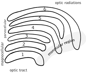
Six layers in the LGN
https://en.wikipedia.org/wiki/Lateral_geniculate_nucleus
Scheme of the optic tract with image being decomposed on the way, up to simple cortical cells (simplified).

Visual pathway lesions From top to bottom: 1. Complete loss of vision, right eye 2. Bitemporal hemianopia 3. Homonymous hemianopsia 4. Quadrantanopia 5&6. Quadrantanopia with macular sparing

This diagram linearly (unless otherwise mentioned) tracks the projections of all known structures that allow for vision to their relevant endpoints in the human brain. Click to enlarge the image.
https://en.wikipedia.org/wiki/Visual_system#
https://en.wikipedia.org/wiki/Artificial_organ
https://en.wikipedia.org/wiki/Pattern_recognition
https://en.wikipedia.org/wiki/Organ-on-a-chip
Cartilage does not contain blood vessels or nerves.
https://en.wikipedia.org/wiki/Cartilage
Chondrification (also known as chondrogenesis) is the process by which cartilage is formed from condensed mesenchyme tissue, which differentiates into chondroblasts and begins secreting the molecules (aggrecan and collagen type II) that form the extracellular matrix. In all vertebrates, cartilage is the main skeletal tissue in early ontogenetic stages;[3][4] in osteichthyans, many cartilaginous elements subsequently ossify through endochondral and perichondral ossification.[5]
Following the initial chondrification that occurs during embryogenesis, cartilage growth consists mostly of the maturing of immature cartilage to a more mature state. The division of cells within cartilage occurs very slowly, and thus growth in cartilage is usually not based on an increase in size or mass of the cartilage itself.[6] It has been identified that non-coding RNAs (e.g. miRNAs and long non-coding RNAs) as the most important epigenetic modulators can affect the chondrogenesis. This also justifies the non-coding RNAs' contribution in various cartilage-dependent pathological conditions such as arthritis, and so on.[7] 
There are three different types of cartilage: elastic (A), hyaline (B), and fibrous (C). In elastic cartilage, the cells are closer together creating less intercellular space. Elastic cartilage is found in the external ear flaps and in parts of the larynx. Hyaline cartilage has fewer cells than elastic cartilage; there is more intercellular space. Hyaline cartilage is found in the nose, ears, trachea, parts of the larynx, and smaller respiratory tubes. Fibrous cartilage has the fewest cells so it has the most intercellular space. Fibrous cartilage is found in the spine and the menisci.
https://en.wikipedia.org/wiki/Cartilage
Chondrogenesis is the process by which cartilage is developed.[1]
Cartilage in fetal development
In embryogenesis, the skeletal system is derived from the mesoderm germ layer. Chondrification (also known as chondrogenesis) is the process by which cartilage is formed from condensed mesenchyme tissue,[2] which differentiates into chondrocytes and begins secreting the molecules that form the extracellular matrix.
Early in fetal development, the greater part of the skeleton is cartilaginous. This temporary cartilage is gradually replaced by bone (Endochondral ossification), a process that ends at puberty. In contrast, the cartilage in the joints remains unossified during the whole of life and is, therefore, permanent.[citation needed]
https://en.wikipedia.org/wiki/Chondrogenesis
https://en.wikipedia.org/wiki/Embryo#Development
https://en.wikipedia.org/wiki/Neuroectoderm
https://en.wikipedia.org/wiki/Neurulation
https://en.wikipedia.org/wiki/Neural_crest
https://en.wikipedia.org/wiki/Surface_ectoderm
https://en.wikipedia.org/wiki/Splanchnopleuric_mesenchyme
https://en.wikipedia.org/wiki/Axial_mesoderm
Chondrogenesis is the process by which cartilage is developed.[1]
Cartilage in fetal development
In embryogenesis, the skeletal system is derived from the mesoderm germ layer. Chondrification (also known as chondrogenesis) is the process by which cartilage is formed from condensed mesenchyme tissue,[2] which differentiates into chondrocytes and begins secreting the molecules that form the extracellular matrix.
Early in fetal development, the greater part of the skeleton is cartilaginous. This temporary cartilage is gradually replaced by bone (Endochondral ossification), a process that ends at puberty. In contrast, the cartilage in the joints remains unossified during the whole of life and is, therefore, permanent.[citation needed]
Mineralization
Adult hyaline articular cartilage is progressively mineralized at the junction between cartilage and bone. It is then termed articular calcified cartilage. A mineralization front advances through the base of the hyaline articular cartilage at a rate dependent on cartilage load and shear stress. Intermittent variations in the rate of advance and mineral deposition density of the mineralizing front, lead to multiple "tidemarks" in the articular calcified cartilage.[citation needed]
Adult articular calcified cartilage is penetrated by vascular buds, and new bone produced in the vascular space in a process similar to endochondral ossification at the physis. A cement line demarcates articular calcified cartilage from subchondral bones.[citation needed]
Repair
Once damaged, cartilage has limited repair capabilities. Because chondrocytes are bound in lacunae, they cannot migrate to damaged areas. Also, because hyaline cartilage does not have a blood supply, the deposition of new matrix is slow. Damaged hyaline cartilage is usually replaced by fibrocartilage scar tissue. Over the last years, surgeons and scientists have elaborated a series of cartilage repair procedures that help to postpone the need for joint replacement.[citation needed]
In a 1994 trial, Swedish doctors repaired damaged knee joints by implanting cells cultured from the patient's own cartilage. In 1999 US chemists created an artificial liquid cartilage for use in repairing torn tissue. The cartilage is injected into a wound or damaged joint and will harden with exposure to ultraviolet light.[3]
Synthetic cartilage
Researchers say their lubricating layers of "molecular brushes" can outperform nature under the highest pressures encountered within joints, with potentially important implications for joint replacement surgery.[4] Each 60-nanometre-long brush filament has a polymer backbone from which small molecular groups stick out. Those synthetic groups are very similar to the lipids found in cell membranes.
"In a watery environment, each of these molecular groups attracts up to 25 water molecules through electrostatic forces, so the filament as a whole develops a slick watery sheath. These sheathes ensure that the brushes are lubricated as they rub past each other, even when firmly pressed together to mimic the pressures at bone joints."[4]
Known as double-network hydrogels, the incredible strength of these new materials was a happy surprise when first discovered by researchers at Hokkaido in 2003. Most conventionally prepared hydrogels - materials that are 80 to 90 percent water held in a polymer network - easily break apart like a gelatin. The Japanese team serendipitously discovered that the addition of a second polymer to the gel made them so tough that they rivaled cartilage - tissue which can withstand the abuse of hundreds of pounds of pressure.[5]
Molecular level
Bone morphogenetic proteins are growth factors released during embryonic development to induce condensation and determination of cells, during chondrogenesis.[6] Noggin, a developmental protein, inhibits chondrogenesis by preventing condensation and differentiation of mesenchymal cells.[6]
The molecule sonic hedgehog (Shh) modifies the activation of the L-Sox5, Sox6, Sox9 and Nkx3.2. Sox9 and Nkx3.2 induce each other in a positive feedback loop where Nkx3.2 inactivates a Sox9 inhibitor. This loop is supported by BMP expression. The expression of Sox9 induces the expression of BMP, which causes chondrocytes to proliferate and differentiate.[7]
L-Sox5 and Sox6 share this common role with Sox9. L-Sox5 and Sox6 are thought to induce the activation of the Col2a1 and the Col11a2 genes, and to repress the expression of Cbfa1, a marker for late stage Chondrocytes. L-Sox5 is also thought to be involved primarily in embryonic chondrogenesis, while Sox6 is thought to be involved in post-natal chondrogenesis.[8]
The molecule Indian hedgehog (Ihh) is expressed by prehypertrophic chondrocytes. Ihh stimulates chondrocyte proliferation and regulates chondrocyte maturation by maintaining the expression of PTHrP. PTHrP acts as a patterning molecule, determining the position in which the chondrocytes initiate differentiation.[9]
Research is still ongoing and novel transcription factors, such as ATOH8 and EBF1, are added to the list of genes that regulate chondrogenesis.[10]
Sulfation
The SLC26A2 is a sulfate transporter. Defects result in several forms of osteochondrodysplasia.[11]
References
Chondrogenesis at the U.S. National Library of Medicine Medical Subject Headings (MeSH)
DeLise, A.M.; Fischer, L.; Tuan, R.S. (September 2000). "Cellular interactions and signaling in cartilage development". Osteoarthritis and Cartilage. 8 (5): 309–34. doi:10.1053/joca.1999.0306. PMID 10966838.
"Dictionary, Encyclopedia and Thesaurus - the Free Dictionary".
"Artificial cartilage performs better than the real thing".
"Study of Tough Hydrogel for Synthetic Cartilage Replacement". Archived from the original on 2009-01-03. Retrieved 2010-06-11.
Pizette, Sandrine; Niswander, Lee (March 2000). "BMPs Are Required at Two Steps of Limb Chondrogenesis: Formation of Prechondrogenic Condensations and Their Differentiation into Chondrocytes". Developmental Biology. 219 (2): 237–49. doi:10.1006/dbio.2000.9610. PMID 10694419.
Zeng, L. (1 August 2002). "Shh establishes an Nkx3.2/Sox9 autoregulatory loop that is maintained by BMP signals to induce somitic chondrogenesis". Genes & Development. 16 (15): 1990–2005. doi:10.1101/gad.1008002. PMC 186419. PMID 12154128.
Smits, Patrick; Li, Ping; Mandel, Jennifer; Zhang, Zhaoping; Deng, Jian Ming; Behringer, Richard R; de Crombrugghe, Benoit; Lefebvre, Véronique (August 2001). "The Transcription Factors L-Sox5 and Sox6 Are Essential for Cartilage Formation". Developmental Cell. 1 (2): 277–290. doi:10.1016/S1534-5807(01)00003-X. PMID 11702786.
St-Jacques, Benoit; Hammerschmidt, Matthias; McMahon, Andrew P. (15 August 1999). "Indian hedgehog signaling regulates proliferation and differentiation of chondrocytes and is essential for bone formation". Genes & Development. 13 (16): 2072–86. doi:10.1101/gad.13.16.2072. PMC 316949. PMID 10465785.
Takács, Roland; Vágó, Judit; Póliska, Szilárd; Pushparaj, Peter Natesan; Ducza, László; Kovács, Patrik; Jin, Eun-Jung; Barrett-Jolley, Richard; Zákány, Róza; Matta, Csaba (2023-03-29). "The temporal transcriptomic signature of cartilage formation". Nucleic Acids Research: gkad210. doi:10.1093/nar/gkad210. ISSN 1362-4962. PMID 36987858.
Haila, Siru; Hästbacka, Johanna; Böhling, Tom; Karjalainen–Lindsberg, Marja-Liisa; Kere, Juha; Saarialho–Kere, Ulpu (26 June 2016). "SLC26A2 (Diastrophic Dysplasia Sulfate Transporter) is Expressed in Developing and Mature Cartilage But Also in Other Tissues and Cell Types". Journal of Histochemistry & Cytochemistry. 49 (8): 973–82. doi:10.1177/002215540104900805. PMID 11457925.
v
t
e
Physiology of bone and cartilage
Bone
Bone density
Bone remodeling Bone healing
Bone resorption
Osseointegration
Ossification
Osteolysis
Bone age
Periosteal reaction
Cartilage
Chondrogenesis
Joint
Range of motion
Teeth
Chewing
Cementogenesis
Category: Embryology
https://en.wikipedia.org/wiki/Chondrogenesis
https://en.wikipedia.org/wiki/Phosphorous
NGC 6751Emission nebula
Planetary nebula
A Hubble Space Telescope (HST) image of NGC 6751's inner bubble
Credit: HST/NASA/ESA.
Observation data: J2000.0 epoch
Right ascension 19h 05m 55.6s[1]
Declination −05° 59′ 32.9″[1]
Distance 6,500 ly (2,000[2] pc)
Apparent magnitude (V) 11.9[3]
Apparent dimensions (V) 0.43′
Constellation Aquila
Physical characteristics
Radius 0.4 ly
Absolute magnitude (V) 0.4
Designations Glowing Eye Nebula, GSC 05140-03497, PK 029-05 1, PN Th 1-J, CSI-06-19031, HD 177656, PMN J1905-0559, PN Sa 2-382, EM* CDS 1043, HuLo 1, PN ARO 101, PN G029.2-05.9, GCRV 11549, IRAS 19032-0604, PN VV' 477, SCM 227, GSC2 S3002210353, 2MASX J19055556-0559327, PN VV 219, UCAC2 29903231
See also: Lists of nebulae
NGC 6751, also known as the Glowing Eye Nebula[2] or the Dandelion Puffball Nebula,[citation needed] is a planetary nebula in the constellation Aquila. It is estimated to be about 6,500 light-years (2.0 kiloparsecs) away.[2]
NGC 6751 was discovered by the astronomer Albert Marth on 20 July 1863.[4] John Louis Emil Dreyer, the compiler of the New General Catalogue, described the object as "pretty bright, small".[4] The object was assigned a duplicate designation, NGC 6748.[4][5]
The nebula was the subject of the winning picture in the 2009 Gemini School Astronomy Contest, in which Australian high school students competed to select an astronomical target to be imaged by Gemini.[6]
NGC 6751 is an easy telescopic target for deep-sky observers because its location is immediately southeast of the extremely red-colored cool carbon star V Aquilae.
https://en.wikipedia.org/wiki/NGC_6751
Articular cartilage repair treatment is focused on the restoration of the surface of an articular joint's hyaline cartilage. Over the last few decades, surgeons and researchers have made progress in elaborating surgical cartilage repair interventions. Though these solutions do not perfectly restore the articular cartilage, some of the latest technologies start to bring very promising results in repairing cartilages from traumatic injuries or chondropathies. These treatments are especially targeted for patients who have articular cartilage damage. They provide pain relief, while at the same time slowing down the progression of damage or considerably delaying the joint replacement (knee replacement) surgery. Articular cartilage repair treatments helps patients to return to their original lifestyle with reduced pain, regaining mobility, going back to work, and even practicing sports again.
Different articular cartilage repair procedures
Though the different articular cartilage repair procedures differ in the technologies and surgical techniques used, they all share the same aim to repair articular cartilage whilst keeping options open for alternative treatments in the future. Broadly taken, there are five major types of articular cartilage repair:[citation needed]
Arthroscopic lavage / debridement
Arthroscopic lavage is a "cleaning up" procedure of the knee joint. This short-term solution is not considered as an articular cartilage repair procedure but rather a palliative treatment to reduce pain, mechanical restriction and inflammation. Lavage focuses on removing degenerative articular cartilage flaps and fibrous tissue. The main target groups are patients with very small defects of the articular cartilage.
Marrow stimulation techniques (micro-fracture surgery and others)
Marrow stimulating techniques attempt to solve articular cartilage damage through an arthroscopic procedure. Firstly, the damaged cartilage is drilled or punched until the underlying bone is exposed. By doing this, the subchondral bone is perforated to generate a blood clot within the defect. Studies, however, have shown that marrow stimulation techniques often have insufficiently filled the chondral defect and the repair material is often fibrocartilage (which is not as good mechanically as hyaline cartilage). The blood clot takes about 8 weeks to become fibrous tissue and it takes 4 months to become fibrocartilage. This has implications for the rehabilitation.[citation needed]
Further on, chances are high that after only 1 or 2 years of the surgery symptoms start to return as the fibrocartilage wears away, forcing the patient to reengage in articular cartilage repair. This is not always the case and microfracture surgery is therefore considered to be an intermediate step.[citation needed]
An evolvement of the microfracture technique is the implantation of a collagen membrane onto the site of the microfracture to protect and stabilize the blood clot and to enhance the chondrogenic differentiation of the MSCs. This technique is known as AMIC (Autologous Matrix-Induced Chondrogenesis) and was first published in 2003.[1]
Microfracture techniques show new potential, as animal studies indicate that microfracture-activated skeletal stem-cells form articular cartilage, instead of fibrous tissue, when co-delivered with a combination of BMP2 and VEGF receptor antagonist.[2]
Marrow stimulation augmented with hydrogel implant
A hydrogel implant to help the body regrow cartilage in the knee is currently being studied in U.S. and European clinical trials.[3] Called GelrinC, the implant is made of a synthetic material called polyethylene glycol (PEG) and denatured human fibrinogen protein.[citation needed]
During the standard microfracture procedure, the implant is applied to the cartilage defect as a liquid. It is then exposed to UVA light for 90 seconds, turning it into a solid, soft implant that completely occupies the space of the cartilage defect. The implant is designed to support the formation of hyaline cartilage through a unique guided tissue mechanism. It protects the repair site from infiltration of undesired fibrous tissue while providing the appropriate environment for hyaline cartilage matrix formation. Over six to 12 months, the implant resorbs from its surface inward, enabling it to be gradually replaced with new cartilage.[4][5][6]
Preliminary clinical studies in Europe have shown the implant improves pain and function.[7]
Marrow stimulation augmented with peripheral blood stem cells
A 2011 study reports histologically confirmed hyaline cartilage regrowth in a 5 patient case-series, 2 with grade IV bipolar or kissing lesions in the knee. The successful protocol involves arthroscopic microdrilling/ microfracture surgery followed by postoperative injections of autologous peripheral blood progenitor cells (PBPC's) and hyaluronic acid (HA).[8] PBPC's are a blood product containing mesenchymal stem cells and is obtained by mobilizing the stem cells into the peripheral blood. Khay Yong Saw and his team propose that the microdrilling surgery creates a blood clot scaffold on which injected PBPC's can be recruited and enhance chondrogenesis at the site of the contained lesion. They explain that the significance of this cartilage regeneration protocol is that it is successful in patients with historically difficult-to-treat grade IV bipolar or bone-on-bone osteochondral lesions.[citation needed]
Saw and his team are currently conducting a larger randomized trial and working towards beginning a multicenter study. The work of the Malaysian research team is gaining international attention.[9]
Osteochondral autografts and allografts
This technique/repair requires transplant sections of bone and cartilage.[10] First, the damaged section of bone and cartilage is removed from the joint. Then a new healthy dowel of bone with its cartilage covering is punched out of the same joint and replanted into the hole left from removing the old damaged bone and cartilage. The healthy bone and cartilage are taken from areas of low stress in the joint so as to prevent weakening the joint.[11] Depending on the severity and overall size of the damage multiple plugs or dowels may be required to adequately repair the joint, which becomes difficult for osteochondral autografts. The clinical results may deteriorate over time.[12]
For osteochondral allografts, the plugs are taken from deceased donors. This has the advantage that more osteochondral tissue is available and larger damages can be repaired using either the plug (snowman) technique or by hand carving larger grafts. There are, however, worries on the histocompatibility, though no rejection drugs are required and infection has been shown to be lesser than that of a total knee or hip. Osteochondral allografting using donor cartilage has been used most historically in knees, but is also emerging in hips, ankles, shoulders and elbows. Patients are typically younger than 55, with BMI below 35, and have a desire to maintain a higher activity level that traditional joint replacements would not allow. Advances in tissue preservation and surgical technique are quickly growing this surgery in popularity.
Joint distraction arthroplasty
This technique involves physically separating a joint for a period of time (typically 8–12 weeks) to allow for cartilage regeneration.[13]
Cell-based repairs
Aiming to obtain the best possible results, scientists have striven to replace damaged articular cartilage with healthy articular cartilage. Previous repair procedures, however, always generated fibrocartilage or, at best, a combination of hyaline and fibrocartilage repair tissue. Autologous chondrocyte implantation (ACI) procedures are cell-based repairs that aim to achieve a repair consisting of healthy articular cartilage.[14]
ACI articular cartilage repair procedures take place in three stages. First, cartilage cells are extracted arthroscopically from the patient's healthy articular cartilage that is located in a non load-bearing area of either the intercondylar notch or the superior ridge of the femoral condyles. Then these extracted cells are transferred to an in vitro environment in specialised laboratories where they grow and replicate, for approximately four to six weeks, until their population has increased to a sufficient amount. Finally, the patient undergoes a second surgery where the in vitro chondrocytes are applied to the damaged area. In this procedure, chondrocytes are injected and applied to the damaged area in combination with either a membrane or a matrix structure. These transplanted cells thrive in their new environment, forming new articular cartilage.
Autologous mesenchymal stem cell transplant
For years, the concept of harvesting stem cells and re-implanting them into one's own body to regenerate organs and tissues has been embraced and researched in animal models. In particular, mesenchymal stem cells have been shown in animal models to regenerate cartilage. Recently, there has been a published case report of decrease in knee pain in a single individual using autologous mesenchymal stem cells. An advantage to this approach is that a person's own stem cells are used, avoiding transmission of genetic diseases. It is also minimally invasive, minimally painful and has a very short recovery period. This alternative to the current available treatments was shown not to cause cancer in patients who were followed for 3 years after the procedure.[15]
See also Stem cell transplantation for articular cartilage repair
Drug therapies
While there are no drugs approved for human use, there are multiple drug candidates with goal to change the progression of cartilage degeneration and even repair it. These are usually referred to DMOADs.
The importance of rehabilitation in articular cartilage repair
Rehabilitation following any articular cartilage repair procedure is paramount for the success of any articular cartilage resurfacing technique. The rehabilitation is often long and demanding. The main reason is that it takes a long time for the cartilage cells to adapt and mature into repair tissue. Cartilage is a slow adapting substance. Where a muscle takes approximately 35 weeks to fully adapt itself, cartilage only undergoes 75% adaptation in 2 years. If the rehabilitation period is too short, the cartilage repair might be put under too much stress, causing the repair to fail.
Concerns
New research by Robert Litchfield, September 2008, of the University of Western Ontario concluded that routinely practised knee surgery is ineffective at reducing joint pain or improving joint function in people with osteoarthritis. The researchers did however find that arthroscopic surgery did help a minority of patients with milder symptoms, large tears or other damage to the meniscus — cartilage pads that improve the congruence between femur and tibia bones.[16] Similarly, a 2013 Finnish study found surgery to be ineffective for knee surgery (arthroscopic partial meniscectomy), by comparing to sham treatment.[17]
References
Behrens P., P. (2005). "Matrixgekoppelte Mikrofrakturierung". Arthroskopie. 18 (3): 193–197. doi:10.1007/s00142-005-0316-0. S2CID 30000568.
Murphy, Matthew P.; Koepke, Lauren S.; Lopez, Michael T.; Tong, Xinming; Ambrosi, Thomas H.; Gulati, Gunsagar S.; Marecic, Owen; Wang, Yuting; Ransom, Ryan C.; Hoover, Malachia Y.; Steininger, Holly (October 2020). "Articular cartilage regeneration by activated skeletal stem cells". Nature Medicine. 26 (10): 1583–1592. doi:10.1038/s41591-020-1013-2. ISSN 1546-170X. PMC 7704061. PMID 32807933.
"Pivotal Study to Evaluate the Safety and Efficacy of GelrinC for Treatment of Cartilage Defects - Full Text View - ClinicalTrials.gov". clinicaltrials.gov. Retrieved 2019-01-23.
Wechsler, Roni; Seliktar, Dror; Sarig-Nadir, Offra; Kupershmit, Ilana; Shachaf, Yonatan; Cohen, Shlomit; Goldshmid, Revital (2015-09-28). "Steric Interference of Adhesion Supports In-Vitro Chondrogenesis of Mesenchymal Stem Cells on Hydrogels for Cartilage Repair". Scientific Reports. 5: 12607. Bibcode:2015NatSR...512607G. doi:10.1038/srep12607. ISSN 2045-2322. PMC 4585928. PMID 26411496.
Berdichevski, Alexandra; Shachaf, Yonatan; Wechsler, Roni; Seliktar, Dror (2015-02-01). "Protein composition alters in vivo resorption of PEG-based hydrogels as monitored by contrast-enhanced MRI". Biomaterials. 42: 1–10. doi:10.1016/j.biomaterials.2014.11.015. ISSN 0142-9612. PMID 25542788.
Korner, A.; Zbyn, S.; Juras, V.; Mlynarik, V.; Ohel, K.; Trattnig, S. (2015-12-01). "Morphological and compositional monitoring of a new cell-free cartilage repair hydrogel technology â€" GelrinC by MR using semi-quantitative MOCART scoring and quantitative T2 index and new zonal T2 index calculation". Osteoarthritis and Cartilage. 23 (12): 2224–2232. doi:10.1016/j.joca.2015.07.007. ISSN 1063-4584. PMID 26187572.
K.F. Almqvist, B.J. Cole, J. Bellemans, R. Arbel, E. Basad, S. Anders, S. Trattnig, A. Korner. The Treatment of Cartilage Defects of the Knee with Microfracture augmented with a Biodegradable Scaffold: Clinical Outcome. Presented at ICRS - Izmir 2013. http://www.regentis.co.il/files/files/ICRS%202013%20Cole%20.pdf
Saw, KY; Anz A; Merican S; Tay YG; Ragavanaidu K; Jee CS; McGuire DA (19 Feb 2011). "Articular cartilage regeneration with autologous peripheral blood progenitor cells and hyaluronic Acid after arthroscopic subchondral drilling: a report of 5 cases with histology". Arthroscopy. 27 (4): 493–506. doi:10.1016/j.arthro.2010.11.054. PMID 21334844.
Wey Wen, Lim. "Generating New Cartilage". The Star. Retrieved 6 May 2011.
Martin, J. Ryan; Sierra, Rafael J. (2017), "Autologous Osteochondral Transfer for Management of Femoral Head Osteonecrosis", Osteonecrosis of the Femoral Head, Cham: Springer International Publishing, pp. 141–156, doi:10.1007/978-3-319-50664-7_14, ISBN 978-3-319-50662-3, retrieved 2022-07-26
Gobezie R, Dubrow S. Arthroscopic total shoulder resurfacing with osteochondral allograft. J Med Ins. 2014;2014(1). doi:https://doi.org/10.24296/jomi/1
Solheim E, Hegna J, Øyen J, Austgulen OK, Harlem T, Strand T. Osteochondral autografting (mosaicplasty) in articular cartilage defects in the knee: results at 5 to 9 years. Knee. 2010 Jan;17(1):84–7.
"Joint-Sparing Alternative to Ankle Fusion or Replacement | HSS". Hospital for Special Surgery. Retrieved 2021-10-21.
Knutsen G, Drogset JO, Engebretsen L, Grøntvedt T, Isaksen V, Ludvigsen TC, Roberts S, Solheim E, Strand T, Johansen O. A randomized trial comparing autologous chondrocyte implantation with microfracture. Findings at five years. J Bone Joint Surg Am. 2007 Oct;89(10):2105–12.
Centeno CJ, Schultz JR, Cheever M, Robinson B, Freeman M, Marasco W (2010). "Safety and Complications Reporting on the Re-implantation of Culture-Expanded Mesenchymal Stem Cells using Autologous Platelet Lysate Technique". Current Stem Cell Research & Therapy. 5 (1): 81–93. doi:10.2174/157488810790442796. PMID 19951252. S2CID 20901900.
Therapy for arthritic knees often as effective as surgery: study
Sihvonen, R.; Paavola, M.; Malmivaara, A.; Itälä, A.; Joukainen, A.; Nurmi, H.; Kalske, J.; Järvinen, T. L. N.; Finnish Degenerative Meniscal Lesion Study (FIDELITY) Group (2013). "Arthroscopic Partial Meniscectomy versus Sham Surgery for a Degenerative Meniscal Tear". New England Journal of Medicine. 369 (26): 2515–2524. doi:10.1056/NEJMoa1305189. PMID 24369076. summary
v
t
e
Procedures involving bones and joints
Orthopedic surgery
Bones
Face
Jaw reduction
Orthognathic surgery
Chin augmentation
Spine
Coccygectomy
Laminotomy
Laminectomy
Laminoplasty
Corpectomy
Facetectomy
Foraminotomy
Vertebral fixation
Vertebral augmentation
Arm
Acromioplasty
Leg
Femoral head ostectomy
Astragalectomy
Distraction osteogenesis
Ilizarov apparatus
Phemister graft
General
Ostectomy
Bone grafting
Osteotomy
Epiphysiodesis
Reduction
Internal fixation
External fixation
Tension band wiring
Cartilage
Articular cartilage repair Microfracture surgery
Knee cartilage replacement therapy
Autologous chondrocyte implantation
Joints
Spine
Arthrodesis Spinal fusion
Intervertebral discs Discectomy
Annuloplasty
Arthroplasty
Arm
Shoulder surgery Shoulder replacement
Bankart repair
Weaver–Dunn procedure
Ulnar collateral ligament reconstruction
Hand surgery Brunelli procedure
Finger joint replacement
Leg
Hip resurfacing
Hip replacement
Rotationplasty
Anterior cruciate ligament reconstruction
Knee replacement/Unicompartmental knee arthroplasty
Ankle fusion
Ankle replacement
Broström procedure
Triple arthrodesis
General
Arthrotomy
Arthroplasty
Synovectomy
Arthroscopy
Joint replacement
imaging: Arthrogram
Arthrocentesis
Arthroscopic lavage
Category: Orthopedic surgical procedures
https://en.wikipedia.org/wiki/Articular_cartilage_repair
Anterior cruciate ligament reconstruction (ACL reconstruction) is a surgical tissue graft replacement of the anterior cruciate ligament, located in the knee, to restore its function after an injury.[1] The torn ligament can either be removed from the knee (most common), or preserved (where the graft is passed inside the preserved ruptured native ligament) before reconstruction through an arthroscopic procedure. ACL repair is also a surgical option. This involves repairing the ACL by re-attaching it, instead of performing a reconstruction. Theoretical advantages of repair include faster recovery[2] and a lack of donor site morbidity, but randomised controlled trials and long-term data regarding re-rupture rates using contemporary surgical techniques are lacking.
https://en.wikipedia.org/wiki/Anterior_cruciate_ligament_reconstruction
Arthroplasty (literally "[re-]forming of joint") is an orthopedic surgical procedure where the articular surface of a musculoskeletal joint is replaced, remodeled, or realigned by osteotomy or some other procedure. It is an elective procedure that is done to relieve pain and restore function to the joint after damage by arthritis or some other type of trauma.
https://en.wikipedia.org/wiki/Arthroplasty
An intervertebral disc (or intervertebral fibrocartilage) lies between adjacent vertebrae in the vertebral column. Each disc forms a fibrocartilaginous joint (a symphysis), to allow slight movement of the vertebrae, to act as a ligament to hold the vertebrae together, and to function as a shock absorber for the spine.
An intervertebral disc (or intervertebral fibrocartilage) lies between adjacent vertebrae in the vertebral column. Each disc forms a fibrocartilaginous joint (a symphysis), to allow slight movement of the vertebrae, to act as a ligament to hold the vertebrae together, and to function as a shock absorber for the spine.
Structure

| Intervertebral disc | |
|---|---|
 Intervertebral disc | |
| Details | |
| Part of | Vertebral column |
| System | Musculoskeletal system |
| Function | Fibrocartilaginous joint between spinal vertebrae |
| Identifiers | |
| Latin | Discus intervertebralis |
| MeSH | D007403 |
| TA98 | A03.2.02.003 |
| TA2 | 1684 |
| FMA | 10446 |
| Anatomical terminology | |
https://en.wikipedia.org/wiki/Intervertebral_disc
Oncotic pressure, or colloid osmotic-pressure, is a type of osmotic pressure induced by the plasma proteins, notably albumin,[1] in a blood vessel's plasma (or any other body fluid such as blood and lymph) that causes a pull on fluid back into the capillary. Participating colloids displace water molecules, thus creating a relative water molecule deficit with water molecules moving back into the circulatory system within the lower venous pressure end of capillaries.
It has the opposing effect of both hydrostatic blood pressure pushing water and small molecules out of the blood into the interstitial spaces within the arterial end of capillaries and interstitial colloidal osmotic pressure. These interacting factors determine the partition balancing of extracellular water between the blood plasma and outside the blood stream.
Oncotic pressure strongly affects the physiological function of the circulatory system. It is suspected to have a major effect on the pressure across the glomerular filter. However, this concept has been strongly criticised and attention has been shifted to the impact of the intravascular glycocalyx layer as the major player.[2][3][4][5]

Above, we see a representation of fluid flow in the presence of colloids, with the left side representing surrounding tissues and the right representing whole blood. The presence of colloids can increase the flow towards the high concentration of colloids by creating colloid osmotic pressure in an otherwise state of equilibrium.
Physiological impact
In tissues, physiological disruption can arise with decreased oncotic pressure, which can be determined using blood tests for protein concentration.
Decreased colloidal osmotic pressure, most notably seen in hypoalbuminemia, can cause edema and decrease in blood volume as fluid is not reabsorbed into the bloodstream. Colloid pressure in these cases can be lost due to a number of different factors, but primarily decreased colloid production or increased loss of colloids through glomerular filtration.[6][9] This low pressure often correlates with poor surgical outcomes.[10]
In the clinical setting, there are two types of fluids that are used for intravenous drips: crystalloids and colloids. Crystalloids are aqueous solutions of mineral salts or other water-soluble molecules. Colloids contain larger insoluble molecules, such as gelatin. There is some debate concerning the advantages and disadvantages of using biological vs. synthetic colloid solutions.[11] Oncotic pressure values are approximately 290 mOsm per kg of water, which slightly differs from the osmotic pressure of the blood that has values approximating 300 mOsm /L.[citation needed] These colloidal solutions are typically used to remedy low colloid concentration, such as in hypoalbuminemia, but is also suspected to assist in injuries that typically increase fluid loss, such as burns.[12]
https://en.wikipedia.org/wiki/Oncotic_pressure
https://en.wikipedia.org/wiki/Kidney
https://en.wikipedia.org/wiki/List_of_surgical_procedures
https://en.wikipedia.org/wiki/Hepatectomy
Techniques include the use of microsurgery, laser, electrocautery, hydrodissection, mechanical dissection, and use of surgical stents, hoods, adhesions barriers, and more.[citation needed]
https://en.wikipedia.org/wiki/Tuboplasty
https://en.wikipedia.org/wiki/Microtube
https://en.wikipedia.org/wiki/Microtubule
https://en.wikipedia.org/wiki/Polymer
A polymer (/ˈpɒlɪmər/;[4][5] Greek poly-, "many" + -mer, "part") is a substance or material consisting of very large molecules called macromolecules, composed of many repeating subunits.[6] Due to their broad spectrum of properties,[7] both synthetic and natural polymers play essential and ubiquitous roles in everyday life.[8] Polymers range from familiar synthetic plastics such as polystyrene to natural biopolymers such as DNA and proteins that are fundamental to biological structure and function. Polymers, both natural and synthetic, are created via polymerization of many small molecules, known as monomers. Their consequently large molecular mass, relative to small molecule compounds, produces unique physical properties including toughness, high elasticity, viscoelasticity, and a tendency to form amorphous and semicrystalline structures rather than crystals.
The term "polymer" derives from the Greek word πολύς (polus, meaning "many, much") and μέρος (meros, meaning "part"). The term was coined in 1833 by Jöns Jacob Berzelius, though with a definition distinct from the modern IUPAC definition.[9][10] The modern concept of polymers as covalently bonded macromolecular structures was proposed in 1920 by Hermann Staudinger,[11] who spent the next decade finding experimental evidence for this hypothesis.[12]
Polymers are studied in the fields of polymer science (which includes polymer chemistry and polymer physics), biophysics and materials science and engineering. Historically, products arising from the linkage of repeating units by covalent chemical bonds have been the primary focus of polymer science. An emerging important area now focuses on supramolecular polymers formed by non-covalent links. Polyisoprene of latex rubber is an example of a natural polymer, and the polystyrene of styrofoam is an example of a synthetic polymer. In biological contexts, essentially all biological macromolecules—i.e., proteins (polyamides), nucleic acids (polynucleotides), and polysaccharides—are purely polymeric, or are composed in large part of polymeric components.
https://en.wikipedia.org/wiki/Polymer
https://en.wikipedia.org/wiki/Cellulose
Hemoglycin (previously termed hemolithin) is a space polymer that is the first polymer of amino acids found in meteorites.[2][3][4]
| Hemoglycin | ||
|---|---|---|
| (Glycine-containing space polymer of amino acids found in meteorites) | ||
 Hemoglycin was found in Acfer 086, an Allende meteorite similar to that pictured. | ||
| Function | unknown, although possibly able to split water to hydroxyl and hydrogen moieties[1] | |
|
| ||
https://en.wikipedia.org/wiki/Hemoglycin
https://www.physio-pedia.com/Cartilage
https://www.thalesgroup.com/en/markets/digital-identity-and-security/government/inspired/biometrics
https://webbtelescope.org/news/webb-science-writers-guide/webbs-scientific-instruments
https://www.google.com/url?sa=t&rct=j&q=&esrc=s&source=web&cd=&ved=2ahUKEwiQjJfr-uv-AhWqj4kEHfLcBxU4KBAWegQICBAB&url=https%3A%2F%2Fwww.diva-portal.org%2Fsmash%2Fget%2Fdiva2%3A1007448%2FFULLTEXT01.pdf&usg=AOvVaw1JsDg1u_0KyMMCSRMGKOYD
No comments:
Post a Comment